
Easy Chaos with Pluto
Simply Making a Mess of Everything
Ask NotebookLMUnderstanding the Predictably Unpredictable
Have you ever wondered why weather forecasts become unreliable beyond a few days? Or why your heart beats with slight irregularities even when you’re perfectly healthy? These phenomena share a fascinating common thread: chaos theory, a branch of mathematics that explains how tiny changes can lead to dramatically different outcomes.
Chaos theory isn’t just an academic curiosity - it’s everywhere around us. From the turbulent flow of water from your faucet to the fluctuations in financial markets, from the patterns of animal populations to the spread of epidemics, chaos theory helps us understand complex systems that at first glance appear random but actually follow hidden patterns.
In this interactive tutorial, we’ll use Pluto notebooks and Julia programming to explore chaos theory hands-on. You’ll discover how simple mathematical rules can generate surprisingly complex behavior, and learn why some systems are fundamentally unpredictable despite being completely deterministic.
Learning Objectives
By the end of this tutorial, you will be able to:
- Set up and use Pluto notebooks for interactive mathematical exploration
- Understand how linear systems behave differently from chaotic ones
- Visualize and analyze the behavior of the logistic function
- Interpret phase portraits and autocorrelation plots
- Recognize sensitive dependence on initial conditions, a key feature of chaos
- Apply these concepts to understand real-world chaotic systems
No advanced mathematics or programming experience is required - just bring your curiosity about how complexity emerges from simplicity.
Getting Started with Pluto
Pluto is a notebook environment for Julia. Install Julia and start it to get a command window. The first step is to add some packages we’ll use for this project. Type ”]” at the prompt (without the quotes) to enter the package manager. The packages you’ll need are:
add Pluto
add PlutoUI
add Plots
add StatsBase
It may take a few minutes as Julia checks and downloads all necessary dependencies. When everything has finished, type “Ctrl-C” to exit the package manager. In the Julia command window, type “Using Pluto” followed by “Pluto.run()”:
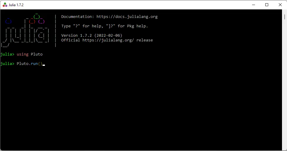
Starting Pluto from the Julia terminal.
A new tab will open in your browser:
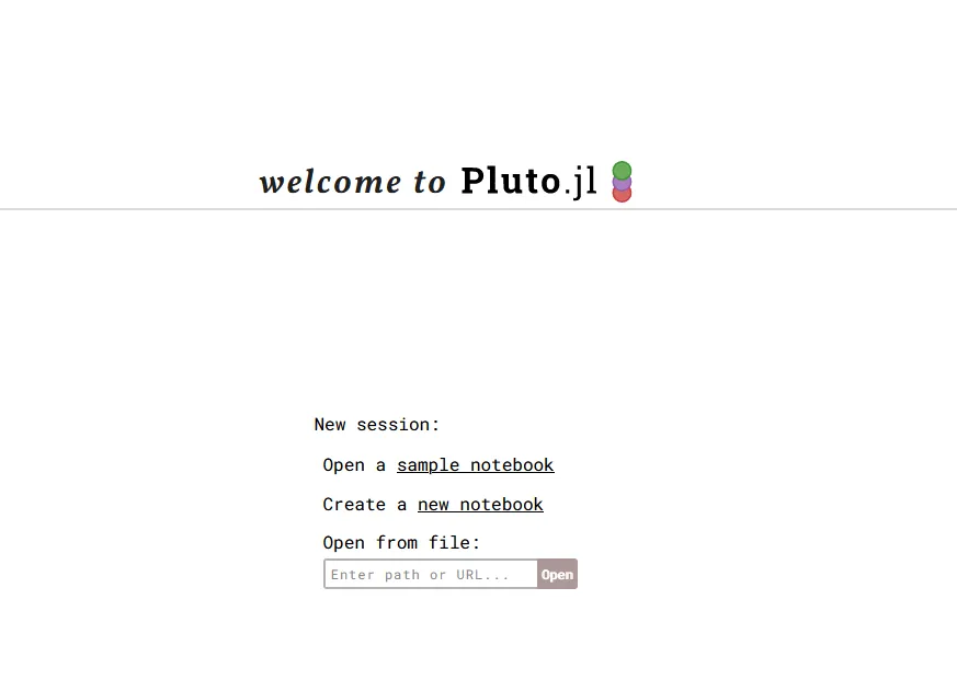
The Pluto notebook.
Download EasyChaos.jl from Github and then enter the path in Pluto below “Open from file:”. The notebook should look very much like the remainder of this post.
Easy Chaos
Pluto is a programming environment for Julia, designed to be interactive and helpful. Changes made anywhere in the notebook affect the entire notebook. Pluto is reactive so you don’t need to recalculate cells.
This is useful in studying chaos because small changes made to a function can have big effects. You can define a function, run it, and immediately see the effects.
A Linear Equation
The equation of a line is where is the slope and is the intercept. The slope is how much changes for each unit change in . For any starting point if you move one step to the right to , the new value becomes . Subtract and all that’s left is .
A step by in the direction gives a change by in the direction, which is the slope of the line.
If , then so the intercept is . Since two points define a line, then start at on the axis, move to and add (or subtract if is negative) to get a second point. Draw your line through the two points.
The line can also be defined as a function,
Let’s start by plotting some lines.
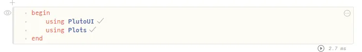
Load libraries into Pluto.
We need a way to change the values of and . First, we’ll make a slider for the slope and set the initial value to . The code for a slider is
@bind m Slider(-5:0.1:5, default=1)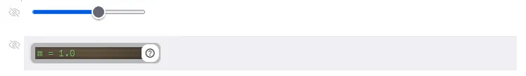
Add a slider.
Next, we’ll make a slider for and set it to . Both can be varied between and .
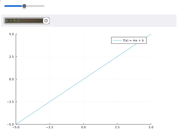
A linear function.
Notice that the origin of the plot is in the center. Move the sliders for and to get a new plot. Interesting, but not chaos.
A Little Chaos
Chaos is doing nearly the same thing over and over and expecting wildly different results. Let’s start with the linear equation above, with and .
Starting at , the output of the function is . Using this new value as the input, . If you do this several times you get the uninteresting sequence
Instead of calculating and then and so on, we can do this in a function iter_f with inputs where is the starting point, and is the number of iterations.
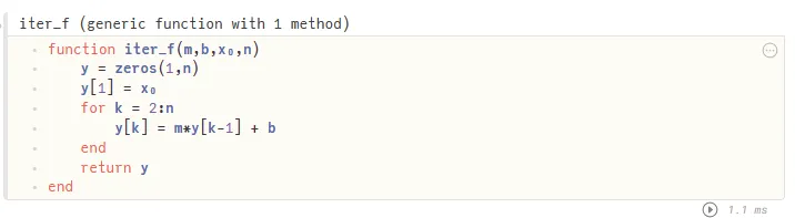
Code for an iterating function.
We can try this function with the equation starting at and for iterations.
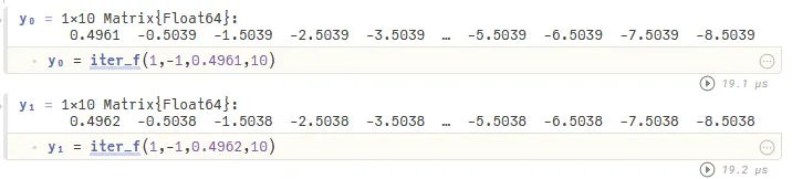
Results after 10 iterations of .
Taking the difference between the outputs gives an uninteresting answer:
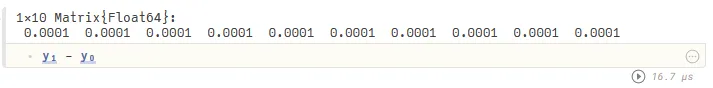
Differences, .
Now, let’s change the equation slightly to , and use the same starting points as before.
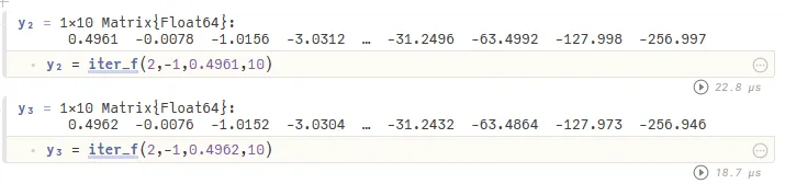
Change the equation to .
The difference between these sequences is:
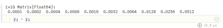
Using the differences double each iteration.
Multiply the differences by to make the changes more obvious:
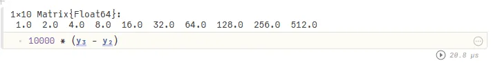
Multiply the differences by to make the change clearer.
This is a little bit surprising, but notice that each number is twice the previous number. It looks like the sequence and could be written as :
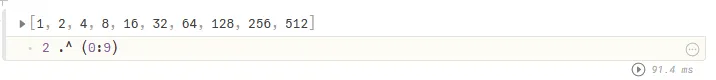
Powers of .
Let’s write out several iterations of in terms of the starting point .
The iterate in terms of is
What happens if we make a small change in ? If we change by a small amount, , then
and the difference between the two results after iterations is (the term with is the same for both)
So long as then we can make as big as we like by iterating enough times, no matter how small is. A small change to the initial value of produces as big a change as you like in the final value, .
There you have it. Chaos!
Even More Chaos
With a slightly more complicated equation, chaos becomes even more interesting. Instead of iterating a linear equation, let’s use the logistic function (see The Growing Gap for an application of logistic functions)
For , this is an inverted parabola that has a maximum at . If you draw the line it intersects the parabola at and . This line is useful for following the iterations or orbits of the function.
Start with a point on the axis, say (point A). Find the value of . This point B is on the parabola above point A.
We want to iterate by using the coordinate of B as the next input. We could calculate and we’ll want to write a Julia function to do that, but it’s also useful to see how the orbit evolves.
Draw a horizontal line until you get to the line at point C. Because C is on the line, then so the coordinates are . The coordinate of C is the coordinate of B, so C becomes the next iterate. From C, draw a vertical line until you intersect the parabola at D which has coordinates .
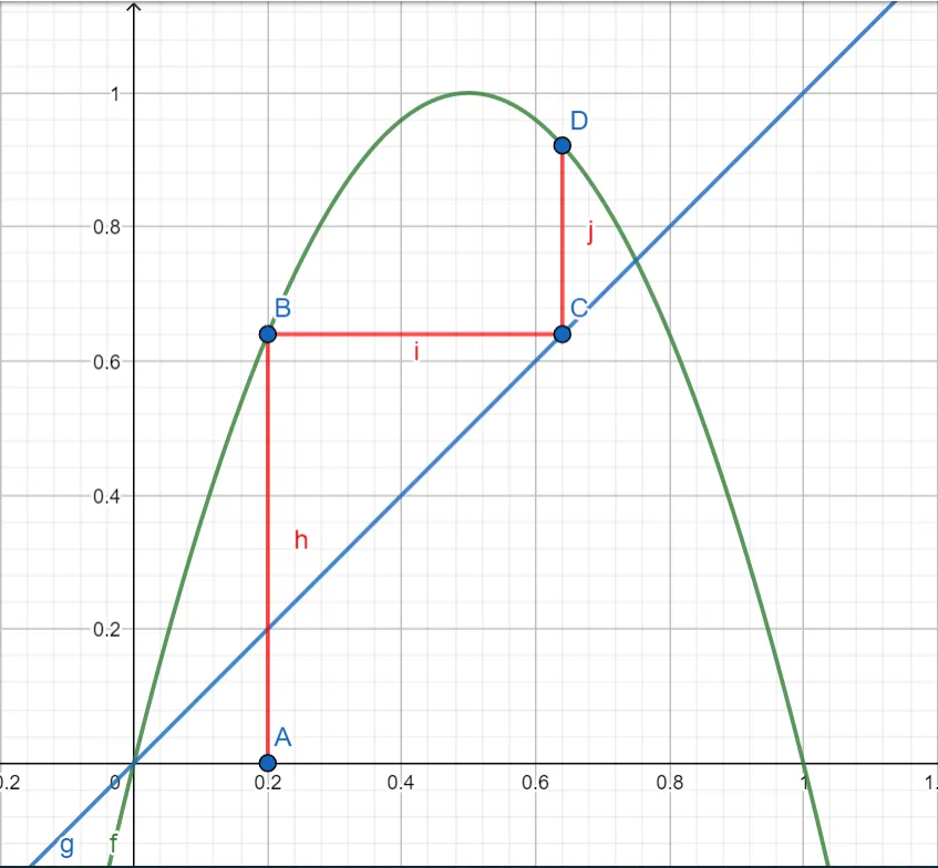
Initial orbits of the logistic function .
This process can be repeated as often as you like and will show the trajectory of the function .
An Iterator for the Logistic Function
Like the iter_f function above, we can write a Julia function to iterate the logistic function. The inputs will be the starting point, , the constant , and the number of iterations with a default value of .
This new function, iter_logistic will return the orbit, .
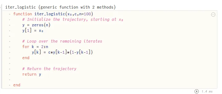
Julia code to output iterates of the logistic function.
Let’s try an example with and .
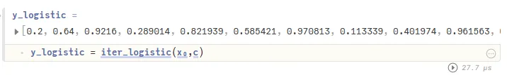
Initial iterates of the logistic function.
Now we can plot the trajectory:
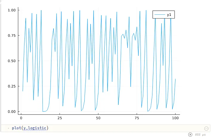
Trajectory of the logistic with .
Try adjusting the value for . When the plot seems pretty chaotic. What happens if you change from to ? This should show that the trajectory is sensitive to the initial value of .
Next, try and set . Is the plot chaotic? Is it sensitive to initial conditions?
Autocorrelation and Orbits
While the plot of the logistic function trajectory for appears chaotic, you might be able to convince yourself that there are repeating patterns. The repetitions are far from identical, but if you imagine making a copy of the plot and shifting it over a bit, it might line up.
This is what autocorrelation does. The amount of the shift is controlled by a lag . For each autocorrelation compares it to . The output of the autocorrelation function is a number between and , where
and is the average of all the ‘s. If then for every , means there is no correlation, and says that .
A orbit is the plot of on the axis and on the axis.
Let’s start by plotting the autocorrelation of the iterated logistic function for different values of .
Rather than scrolling back up to set and , let’s just create two new variables and call them and .
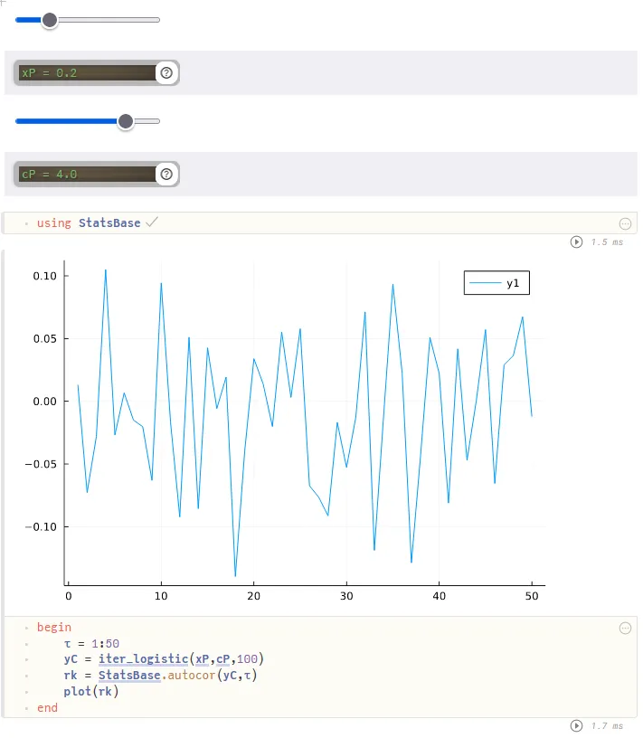
Autocorrelation of the logistic function.
Choose the autocorrelation step :
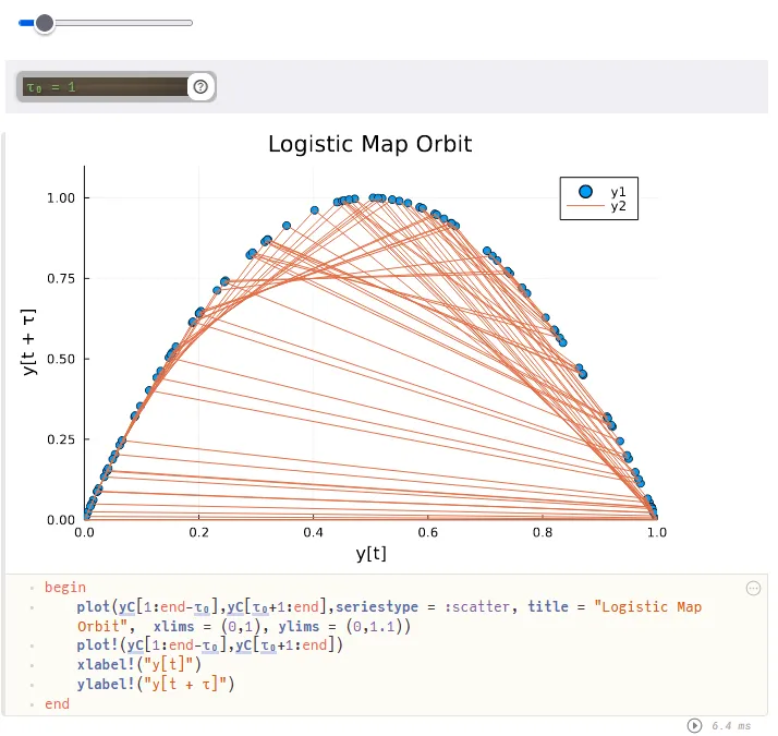
Orbit of the logistic with .
The autocorrelation plot seems about as chaotic as the logistic function, but when , the phase portrait is very smooth. In fact, the outline of the blue dots (y1) looks just like the logistic function!
This should be expected since for every .
Why choose ? That choice of plots the orbit of the function. The orange lines (y2) show which point follows the current location. On the left side, the path seems to be mostly upwards towards a nearby point. On the right, points are sent back to the left half except those near .
Try setting and you’ll see that the orbit becomes the line , because there’s perfect correlation between and . The plot doesn’t provide any insight. Try some other values of to see what happens.
With Pluto, you can change the input values to a function to immediately see the effects.
Code for this article
EasyChaos.jl - A Pluto notebook to do some simple experiments with chaos theory.
Software
- Julia - The Julia Project as a whole is about bringing usable, scalable technical computing to a greater audience: allowing scientists and researchers to use computation more rapidly and effectively; letting businesses do harder and more interesting analyses more easily and cheaply.
- Pluto - Pluto is an environment to work with the Julia programming language.
References and Further Reading
- Autocorrelation Plot. Accessed 6/6/2025.
- Biswas, Hena Rani, Hasan, Maruf, Bala, Shujit Kumar. Chaos theory and its applications in our real life. 2018.
- C, Caitlyn. Chaos Theory for Dummies: Finding Beauty in Disorder. Accessed 6/6/2025.
- Chaos in the machine: How foundation models can make accurate predictions in time-series data | Santa Fe Institute. 2025.
- Chaos Theory. Mathigon. Accessed 6/6/2025.
- Chaos theory. Wikipedia. 2025.
- Dynamical Systems and Chaos - Interview with Stephen H. Kellert > Introduction | Class Central Classroom. Accessed 6/6/2025.
- Explainer: What is chaos theory?. 2023.
- How Mathematicians Make Sense of Chaos. Quanta Magazine. 2022.
- An Introduction to Chaos. Accessed 6/6/2025.
- Lee, Sarah. 5 Essential Steps to Understand Chaos Theory Dynamics. Accessed 6/6/2025.
- Lorenz, Edward N.. Deterministic Nonperiodic Flow. Journal of the Atmospheric Sciences. 20. 130-141. 1963.
- Chaos Theory Simply Explained. ResearchGate. Accessed 6/6/2025.
- Peitgen, Heinz-Otto, Jürgens, Hartmut, Saupe, Dietmar. Chaos and Fractals: New Frontiers of Science. 2004.
- Strogatz, Steven. Nonlinear dynamics and chaos: with applications to physics, biology, chemistry, and engineering. 2019.
- Varniex. Chaos Theory in 13 Minutes. 2025.
- What is Chaos Theory? – Fractal Foundation. Accessed 6/6/2025.
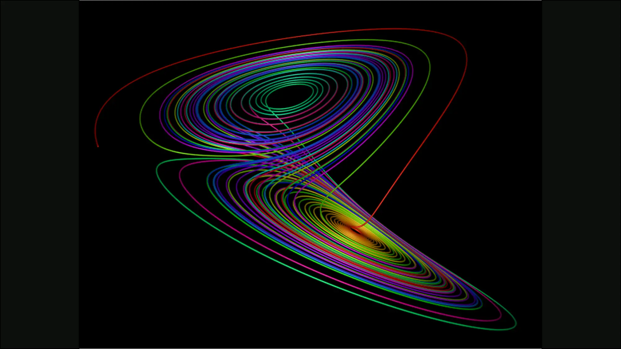
Image credits
Hero image from Introduction to Online Nonstochastic Control, Elad Hazan, Karan Singh, Research Gate, Figure 2.7: Lorenz attractor Nov 2022.