Tools of Chaos
Orbits
Ask NotebookLMHave you ever wondered why weather forecasts become less reliable the further into the future they try to predict? Or why the paths of planets and asteroids can sometimes behave in seemingly random ways? The answer lies in chaos theory - one of the most fascinating intersections of mathematics and natural phenomena.
In this article, we’ll explore the building blocks of chaos using the idea of orbits - the paths that objects or mathematical points take as they evolve over time. With computational tools available in the Julia language and some surprisingly simple equations, we’ll see how predictable rules can generate unpredictable behavior.
Concepts that we’ll cover in this article include:
- The difference between discrete and continuous chaotic systems
- The three key properties that make a system truly chaotic
- How to use Julia programming language and Pluto notebooks to visualize and explore chaotic orbits
- Real-world applications and examples of chaos theory
By the end, you’ll have both an intuitive understanding of chaos theory and the practical tools to begin exploring it yourself. So let’s dive into the fascinating world where simple rules meet complex behavior.
Pluto Orbits
The previous post, Easy Chaos with Pluto showed how to run a Pluto notebook in Julia. A more in-depth introduction is on the MIT open course Introduction to Computational Thinking which describes the first-time setup of Julia and Pluto and provides a Cheatsheets page.
From JuliaDynamics we’ll use ChaosTools, DynamicalSystems, InteractiveDynamics, and DrWatson. You should also add DifferentialEquations, Plots, and GLMakie with Pkg, the Julia package manager.
Download the Pluto notebook, Orbits.jl used for this post.
The Discrete and the Continuous
In chaos theory, an orbit is the sequence generated by repeatedly applying a function to the initial point .
Chaotic orbits may be either discrete or continuous. In the previous post Easy Chaos with Pluto the logistic function
is an example of a discrete system. For and , this formula gives . The sequence is which makes discrete steps between iterations.
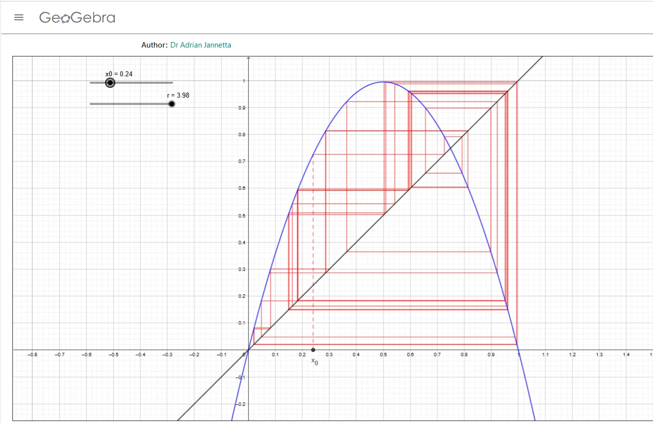
Orbits of the logistic map in Geogebra.
Continuous functions are often written in terms of time, such as the Van der Pol equation
Pick any point . The notation and are the derivatives of and which tells you how fast point is moving. Suppose . Putting those coordinates into the Van der Pol equation gives
which says that the point is moving to the right with velocity , and the velocity is zero. The time variable doesn’t seem to show up, but ) is the velocity of which is a function of time. In some cases, you may see the notation or indicating that velocities are functions of time. The ratio gives the slope of the velocity,
Starting at point , the velocity is , so for some small time step the next position would be . The time step can be as small as you like making the trajectory, or orbit, of a continuous function.
It isn’t too difficult to generate the sequence of points in the orbit of the logistic function, but for the Van der Pol equation the velocity changes with every small time step, so keeping track of the orbit points becomes tedious. Fortunately, computers can handle these kinds of equations and plot the orbits for us.
Chaotic Orbits
Orbits are chaotic if they have the following three properties:
- Sensitive dependence on initial conditions
- Topological transitivity
- Dense periodic orbits
One way to think about these properties is to imagine a car race. At the start they all have slightly different initial conditions. Some engines will be stronger than others, some drivers better than others, and only one car gets the pole position. Each car occupies a slightly different position on the track. These slight differences are the sensitive dependence on initial conditions that will determine the outcome of the race.
When the race starts the cars move down the track and begin to separate, each one completing laps at slightly different times than the others, and the paths that they take may be similar, but each car creates its own path. After enough time, the leaders will begin to lap the stragglers, and even though the cars separated at the start, they’re now back together, which is a little like topological transitivity.
The mathematical definition of topological transitivity says that for any two regions and in the orbit, there is some positive integer such that some of the iterated points in , or can be found in . This holds no matter how small the regions and are, and no matter where they are in the orbit.
Not all of the points in will map into , and not all of the points in will be the result of iterated points in , but there will be at least one point that does map. Another way to think about this is that every point in the orbit approaches every other point through iterations of .
A consequence of topological transitivity is that an orbit is never two or more independent orbits. Even if the orbit appears to have distinct branches, eventually points in one branch will iterate into every other branch.
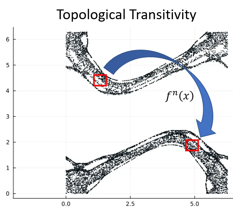
Points in one orbit eventually map to points in every other branch.
A periodic orbit is one where , so comes back to itself after iterations of . The cars go around the track and return to the points where they started. The analogy with race cars isn’t quite accurate because the lateral position on the track changes from lap to lap, but maybe you can imagine the propagation of points to be a little like a car race. Dense periodic orbits mean that at any point in the orbit of one point, you can always find the orbit of another point nearby.
These three properties of chaos were first described by Robert L. Devaney in his book, An Introduction to Chaotic Dynamical Systems. A popular non-mathematical book, Chaos: Making a New Science was published by James Gleick in 1987. Wolfram MathWorld says this about the definition of chaos,
Gleick notes that “No one [of the chaos scientists he interviewed] could quite agree on [a definition of] the word itself,” and so instead gives descriptions from a number of practitioners in the field. For example, he quotes Philip Holmes (apparently defining “chaotic”) as, “The complicated aperiodic attracting orbits of certain, usually low-dimensional dynamical systems.” Similarly, he quotes Bai-Lin Hao describing chaos (roughly) as “a kind of order without periodicity.”
Chaotic systems are deterministic which means there is no random component to an orbit. Given a starting position, in principle, you can calculate exactly where a point will be steps into the future for any value of . What makes them seem random is that two nearby starting points evolve in unpredictable ways.
The Orbits Notebook
The Orbits.jl notebook lets you experiment with both discrete and continuous dynamical systems using both built-in equations and systems you can write yourself. Using a built-in method is as simple as loading the dynamical system rule:
ds_henon = Systems.henon()generating the trajectory
traj*henon = trajectory(ds*henon,100000)and plotting the result
plot(traj*henon[:,1],traj*henon[:,2], seriestype = :scatter, aspect_ratio = :equal)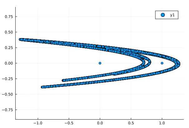
The Hénon Map.
The equations for the Hénon Map are
which could have been written in Julia as
function henon_rule(u, p, n)
  x, y = u # Current state
  α, β = p # Parameters
  xn = 1 - α*x^2 + y
  yn = β*x
  return SVector(xn, yn)
end
After setting the initial condition and the parameter vector , we could generate the trajectory and plot it just as we did with the built-in version. The rule requires a step counter for discrete systems, or a time for continuous systems even if these variables don’t show up in the equations.
The Orbits.jl notebook is fully documented so you should be able to change parameters and extend equations or even create new systems. Have fun experimenting!
Taking Chaos Further
Throughout this article, we’ve explored how simple mathematical rules can generate surprisingly complex and unpredictable behavior. We’ve seen how chaos emerges from both discrete systems like the logistic map and continuous systems like the Van der Pol oscillator. The three key properties - sensitive dependence on initial conditions, topological transitivity, and dense periodic orbits - give us a framework for understanding what makes a system truly chaotic.
But this is just the beginning of what you can explore. Using the provided Pluto notebook, here are some other experiments you might try:
- Modify the parameters of the Hénon map and observe how the orbit structure changes. What happens when you push the parameters to extreme values?
- Compare different initial conditions that are very close together. How many iterations does it take before their orbits become noticeably different?
- Try creating your own discrete dynamical system by writing a simple rule. Can you identify whether it exhibits chaotic behavior?
- Experiment with visualizing orbits in different ways - try color-coding points based on their iteration number or plotting in 3D for systems with three variables.
Hopefully, the tools and concepts we’ve covered here will allow you to continue the mathematical exploration of chaos. Whether you’re interested in weather patterns, population dynamics, or the motion of planets, chaos theory provides insights into the complex behavior of natural systems.
Code for this article
Orbits.jl - A Pluto notebook to study chaos
Software
- Julia - The Julia Project as a whole is about bringing usable, scalable technical computing to a greater audience: allowing scientists and researchers to use computation more rapidly and effectively; letting businesses do harder and more interesting analyses more easily and cheaply.
- Pluto - Pluto is an environment to work with the [Julia programming language](https://julialang.
- DrWatson - DrWatson is a scientific project assistant software.
References and further reading
- Pluto on Github
- DynamicalSystems.jl
- Julia Dynamics
- Chaos, Making a New Science by James Gleick
- An Introduction to Chaotic Dynamical Systems by Robert L. Devaney
- Robert Devaney’s homepage at Boston University
- Santa Fe Institute Complexity Explorer
- Introduction to Dynamical Systems and Chaos course at SFI
- Nonlinear Dynamics videos from SFI
- Wolfram MathWorld Chaos page
- Introduction to Computational Thinking MIT course
- DynamicalSystems.jl examples
- Introduction to DynamicalSystems.jl video
- JuliaDynamics.jl tutorial notebooks
- Creating an instance of a dynamical system, JuliaDynamics
- What to do with a
DynamicalSystem? Orbit Diagram, JuliaDynamics - DynamicalSystems.jl: A Julia software library for chaos and nonlinear dynamics, George Datseris
- CHAOS ON THE INTERVAL a survey of relationship between the various kinds of chaos for continuous interval maps, Sylvie Ruette
- Chaos Definition and Classification, Alexander Coxe
- The logistic map and you, Jaco Stroebel
- Dynamical Systems, Scholarpedia
- Periodic Orbit, Scholarpedia
- Galactic Dynamics, Scholarpedia
- A Gentle Introduction to Chaos Theory, Francesco Di Lallo
- Chaos in the World, Angela Zhao (Discussion and Conclusion)
- Why do chaotic systems need dense periodic orbits?
- Chaos and Randomness, Eric Jang
- Topological transitivity and recurrence as a source of chaos, Constantin P. Niculescu
- On Devaney’s Definition of Chaos and Dense Periodic Orbits, Syahida Che Dzul-Kifli and Chris Good
- Topological Chaos: What may this mean? Francois Blanchard
- Periodic Orbits
- Lecture Notes, Burbulla
- Orbits, Periodic Orbits, and Dense Orbits – Oh My!, Mark Chu-Carroll
- Sarkovsky’s theorem, John D. Cook
- Dynamical System, Wikipedia
- Standard Map, Wikipedia
- Lotka-Volterra Equations, Wikipedia
- Van der Pol oscillator, Wikipedia
Image credits
Hero: Iconic Arecibo Observatory’s 1000-feet telescope is beyond repair, will be demolished amid safety concerns Mihika Basu, MEAWW Nov 19, 2020.