
Recursive Sequences as Linear Transformations
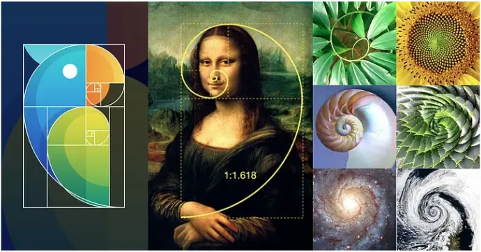
Fibonacci Spirals the Drain
Ask NotebookLMThis problem is from Otto K. Bretscher posted in the Classical Mathematics Facebook group.
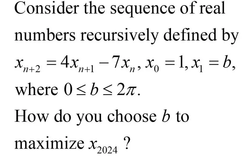
Recursive problem.
We’re working on a new platform for scientific research called eurAIka that combines The Whiteboard for writing notes, equations, and pasting in graphics, The Librarian for AI-assisted literature search, and The Coder where you can write programs. This will be our first attempt at using eurAIka for a Wild Peaches article.
The Fibonacci Sequence
Let’s start with an easier problem, the Fibonacci sequence:

The Fibonacci sequence.
where the recursive relationship is and . We could generalize this to include any sequence composed of multiples of the previous two terms,
The coefficients for the Fibonacci sequence, and for the problem we’re trying to solve and .
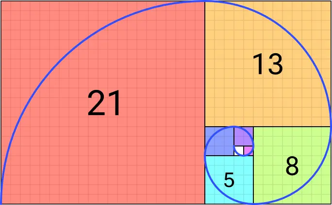
The Fibonacci Spiral.
It wouldn’t be difficult to write a function in a computer language that calculates all of the elements of the sequence up to the one we’re interested in. To see how the value for changes the outcome, we’d have to run the code over many test cases to see what happened.
Another way to get to the value of can be done in one step using linear algebra. Let’s call the vector composed of the first two entries of the sequence, so
The next step in the sequence puts in the first position and moves down giving
The entries of this new vector are linear combinations of the previous two entries of the sequence, so we could define a matrix that multiplies to get
The recursion step says that and so on, or in terms of the original vector, For the Fibonacci sequence, . For example, we can calculate the 16th entry in the sequence by calculating , which gives in the location. A convenient trick to extract just the upper left entry using Julia is to write this as (A^14)[1,1].
If then is called an eigenvector and the constant is an eigenvalue. For the Fibonacci matrix there are two eigenvalues, (the positive one is the golden ratio, ) and if you take the ratio of to you’ll see that it converges to . The other eigenvalue is the negative inverse of the first one, so .
The matrix can be decomposed into where is the array of eigenvectors and is a diagonal array with and on the diagonal. The eigenvectors are unit vectors, so is orthogonal meaning that , the identity matrix. With this decomposition, powers of can be written as
Since is diagonal, then is also diagonal with and on the diagonal, making matrix powers easy to calculate. Now the 15th iterate of can be found from
This is numerically unstable because will quickly overflow or underflow as powers of and approach either zero or but this idea will become theoretically useful for our problem.
As we saw above, the ratios of successive values of the Fibonacci sequence approach the golden ratio, . If you plotted points you would see that they all lie nearly on the line , and the fit gets better the farther out you go. The points are the vectors which when multiplied by give the next point or vector in the sequence.
Geometrically, matrix multiplication transforms vectors through rotation and scaling. What we’re seeing here is that in the decomposition , the first multiplication only performs a rotation since is unitary. The scaling occurs with , and multiplication by restores the direction.
As an example, let so
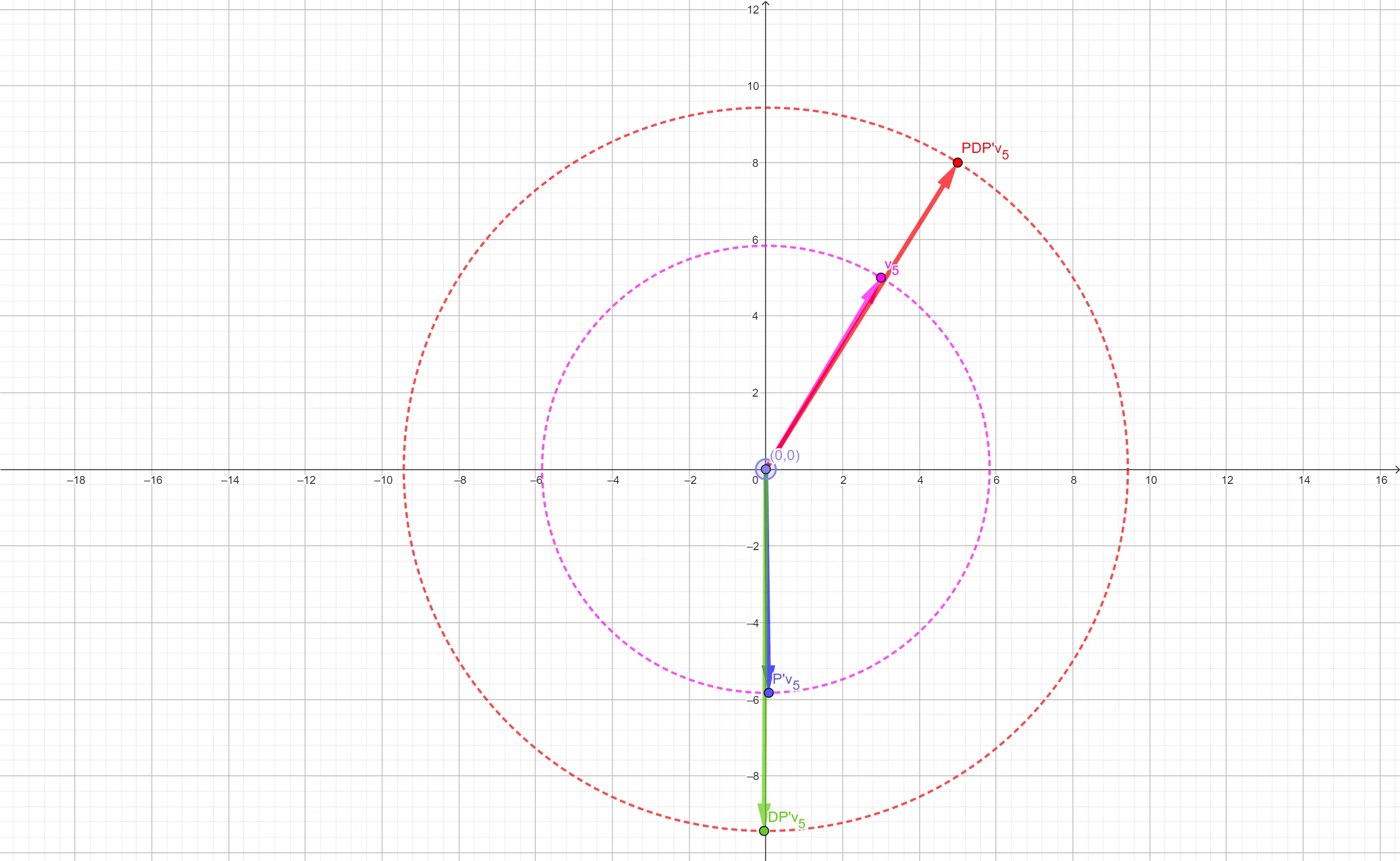
Matrix multiplicaion rotation and scaling effects.
Notice that and lie on the same circle as do the points and showing that is a rotation, while the scaling between and is multiplication by .
The Bretscher Sequence
Now let’s apply this same technique to the Bretscher sequence . Define the transition matrix,
which has the characteristic equation derived from the determinant of
The eigenvectors are found by solving for for some . This gives
Expanding this gives the system of equations,
giving eigenvectors . The inverse of
is
Let be the diagonal matrix formed from the eigenvalues,
and then verify that and , the identity matrix.
For the Fibonacci sequence, the eigenvectors formed an orthonormal basis, so we could quickly calculate powers of the matrix because
The Bretscher matrix also has this property, except that the eigenvectors aren’t orthogonal. Still, the eigenvectors found above form a basis of the space spanned by , so we can still calculate for any power . This wouldn’t be so bad for some small values of , but we’ll need another method to answer the question of how to maximize .
Otto Bretscher says in response to his original question,
The roots of the characteristic polynomial are 2 ± i√3 = √7exp[±i*arctan(√3/2)]. We can write x(n) as a linear combination of (2 + i√3)^n and (2 - i√3)^n and bring this expression into real form. While these computations are straightforward, they are somewhat tedious, perhaps best left to a computing device; the answer provided by WolframAlpha is attached. Since the coefficient of b turns out to be negative for n = 2024, we maximize x(2024) by letting b = 0.
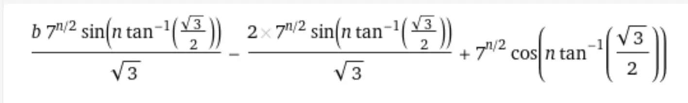
The characterisitic polynomial in Wolfram Alpha.
Pari/GP can calculate numbers with very high precision, so let’s give it a try. The sequence begins , so the next element is found from
The fourth element is so the will be multiplied by . Enter the matrix in PARI/GP as
B = [4, -7; 1, 0]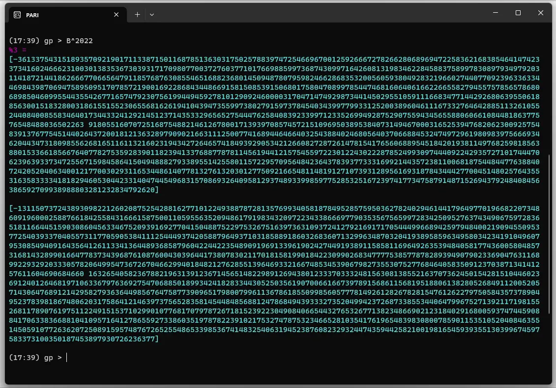
The PARI/GP solution.
So, how do you choose to maximize ? Well you don’t need to know the value of the number that Pari just computed, all you need is the sign. Since the value of the entry in the position of this little matrix is negative, the that maximizes is zero.
Spiraling to the Solution: Where Mathematics Meets Beauty
This exploration of the Bretscher sequence demonstrates how linear algebra can be useful in solving seemingly complex recursive problems. We found that
- Recursive sequences can be reframed as linear transformations using matrices.
- The eigenvalues and eigenvectors of these matrices reveal the long-term behavior of the sequence.
- Complex eigenvalues, as in the Bretscher sequence, create spiral patterns in the sequence behavior.
- Matrix decomposition provides an elegant way to compute high-powered terms .
If you’re interested in exploring further, here are some suggested investigations:
- Experiment with different coefficients in the general sequence and observe how they affect the sequence behavior.
- Create visualizations of how different recursive sequences spiral in the complex plane.
- Investigate what happens when you extend the recursion to depend on three or more previous terms.
- Study how the initial conditions affect the long-term behavior of various recursive sequences.
- Explore connections between recursive sequences and natural phenomena like population growth or wave propagation.
The methods demonstrated here extend beyond just mathematical curiosity - they have applications in fields ranging from financial modeling to quantum mechanics. Understanding how to analyze recursive sequences through linear transformations provides a powerful tool for tackling complex problems in science and engineering.
Recursive image of this problem in eurAIka.
Definitions
Linear combination: If vector for some constants and , then is a linear combination of the two vectors and .
Eigenvector, eigenvalue: If the vector can be written as for some matrix and constant , then is an eigenvector of , and is the associated eigenvalue.
Orthogonal vectors: Vectors are orthogonal if the angle between them is in two or three dimensions. The better definition of orthogonality is that the dot product between the two vectors is zero, and this holds for all dimensions. To calculate the dot product, multiply the elements in one vector by the corresponding element in the second vector and add up the result. If it sums to zero, the vectors are orthogonal.
Orthogonal matrix: A square matrix with real valued elements and with the property that its inverse is equal to its transpose is orthogonal.
Diagonal matrix: All elements not on the main diagonal are zero.
Transition matrix: A matrix that transforms vectors from one basis to another. Also called a change of coordinates matrix.
Characteristic polynomial: The polynomial arising from where is the determinant and is the identity matrix.
Code for this article
Problem2024.ipynb - JupyterLab notebook in Julia
Bretscher_sequence.ipynb - JupyterLab notebook using Wolfram Language 13.2
Fibonacci.html - Geogebra worksheet to demonstrate rotation and scaling effects of linear transformations (open in br)
Software
- Julia - The Julia Project as a whole is about bringing usable, scalable technical computing to a greater audience: allowing scientists and researchers to use computation more rapidly and effectively; letting businesses do harder and more interesting analyses more easily and cheaply.
- JupyterLab - JupyterLab is the latest web-based interactive development environment for notebooks, code, and data.
- Wolfram Language - Wolfram Language is a symbolic language, deliberately designed with the breadth and unity needed to develop powerful programs quickly.
- Pari/GP - PARI/GP is a widely used computer algebra system designed for fast computations in number theory (factorizations, algebraic number theory, elliptic curves, modular forms, L functions.
References and further reading
- Interactive Linear Algebra, Dan Margalit, Joseph Rabinoff. 5.5 Complex Eigenvalues
- Diagonalize a 2 by 2 Matrix and Calculate the Power
- COMPLEX Eigenvalues, Eigenvectors & Diagonalization full example - Dr. Trefor Bazett
- Fibonacci sequence - Wikipedia
- Matrix multiplication - Wikipedia
Image credits
- Hero: How I made money using The Golden Ratio Law of Design this Pandemic
- Problem statement: Otto K. Bretscher
- Fibonacci sequence: Fibonacci sequence - Wikipedia
- Fibonacci spiral: Wikimedia Commons, Fibonacci Spiral over tiled squares
- Rotation and Scaling Effects: Geogebra
- Characteristic Polynomial from Wolfram Alpha: Wolfram Alpha
- PARI Solution: PARI/GP
- Recursive image of this problem in eurAIka: eurAIka