
Investigating Integrals with Geogebra
Solving a problem from the Classical Mathematics Group
Ask NotebookLMHave you ever wondered how mathematicians calculate the area of curved shapes? While finding the area of a rectangle is straightforward - just multiply length by width - what happens when we’re dealing with curves that bend and twist? This is where one of calculus’s most powerful tools comes into play: integration.
In the previous article, CAS with Geogebra we looked at derivatives. Here we’ll go in the opposite direction and investigate integrals. If you have a function then the derivative is written as and gives the slope of the function at any point . Integration reverses this process and gives you from the derivative function .
Integration isn’t just an abstract mathematical concept - it is used in many practical applications. In physics, integrating the velocity of an object gives the total distance travelled, and in engineering you could integrate the height of the water in Lake Mead to determine the force on the Hoover Dam. Mathematically, integration is done by summing up the areas of infinitely many rectangles with infinitesimally small widths. Let’s take a look at how this works with an example.
The Integral
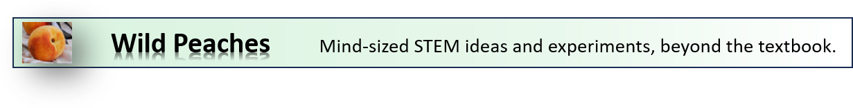
The way the integral is calculated is to find the area of small rectangles under the curve of . Suppose and we want to find the area of a small rectangle centered at that has a width of .
The area under the curve.
Calculating the value of at gives , and since the width of the rectangle is the area is Now imagine repeating this from to along the axis. Add up all of the areas of the rectangles and you’ll get an approximation for the total area under the curve, called the Riemann sum.
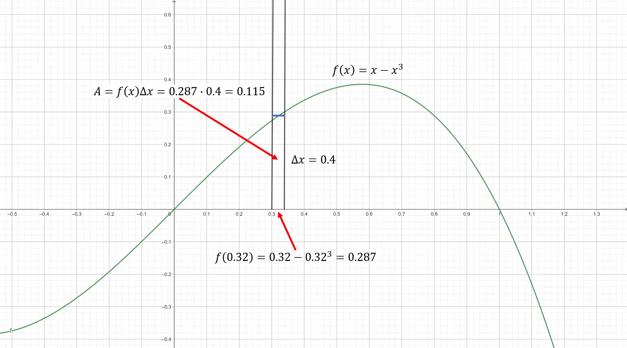
Riemann sums - function integration.
Alexander Bogomolny built an interactive demonstration of Riemann sums on his website Cut the Knot where you can choose several different functions, select left, midpoint, or right ends for the height of the rectangles, and set the width of the rectangles to see how your choices affect the estimated area.
Using the summation symbol we can write
where is the location of the center of the rectangle, and represents the total area.
But, the area under the curve is just a number and the integral is a function. Is this like the wave-particle duality of photons? No, the answer is much simpler. The integral becomes an area if you measure between two points along the axis. In the first example, we might start at and end at . If the curve is above the axis the area is a positive number and if it’s below then the area is negative.
If the beginning and endpoints aren’t given, then the integral is a function. It’s the function that has a derivative , so we’d like a procedure that finds from .
Techniques of Integration
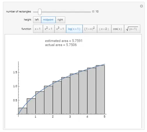
Finding the integral of a function is often tricky and may involve substituting a variable for a term in the function, using rules from trigonometry, or applying something called integration by parts. Sometimes you can find the solution in a table of integrals or you may resort to a computer algebra system like WolframAlpha or the Geogebra CAS. For the cubic polynomial above, Geogebra finds the integral,
Geogebra CAS integral.
The function that is the integral of is
where is called the constant of integration (Geogebra uses ). The integral function looks like
Integral of the cubic function.
which has slope at every point . Since the constant shifts the function up or down the axis it won’t change the shape of the curve, so the derivative remains the same.
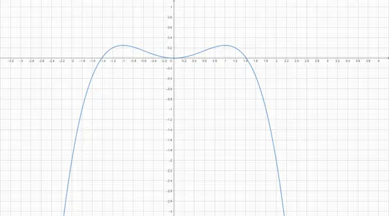
A more difficult integral problem
A problem that requires a bit more thought is this:
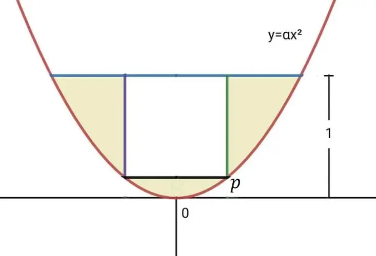
An integral problem: Find the area of the colored region.
What is the area in the colored region? An assumption made by people in the Classical Mathematics group is that the white rectangle is a square, but you know what they say about assumptions - they make an ass out of u and mptions.
Let’s split the area into two pieces. Let be the total area above the curve and below the line , and be the area of the white rectangle. Since the figure is symmetric about the axis, we can start everything at and just double the areas.
To get the area in the colored region , we can calculate the area below and subtract the area below , so . Using the Geogebra CAS, the integral is
From the Fundamental Theorem of Calculus, the area enclosed by over an interval is , or the difference of the integral function at the endpoints of the interval. In this case, and (ignoring the integration constant ) .
What’s the value of ? That is, where does intersect ? It has to be where so at . In mathematical notation,
The integral symbol is used to denote the Riemann sum when the width of the rectangles approaches zero. The line at the end with at the bottom and at the top is the notation to tell us to evaluate the integral at the endpoints. Doing the evaluation gives,
The area in the white rectangle depends on the location of the point , and the area of the rectangle is
The area in the colored region is the difference
If we set , then the area becomes .
.webp)
The area of the colored region as a function of .
Notice that at and the area of the white rectangle is zero and the colored region has area shown by the green line.
One last question is, what is the value of that makes the white rectangle a square, and what is the value of at that point? For the rectangle to be a square the length of the side from to the line must be equal to two times since is only half the length of one side of the square. This means,
Rearranging this equation gives a quadratic,
with solutions
Substituting this into the equation for the area ,
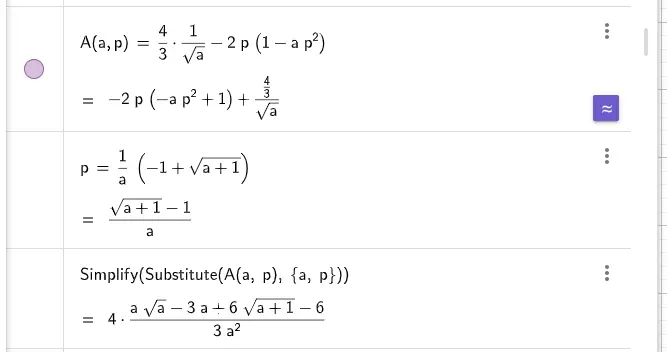
The Geogebra solution.
using the positive root for .
Integrating all the pieces
We’ve seen how integration works through the application of Riemann sums, and how Geogebra can be a useful tool towards solving integral problems. Now that you know how to calculate the integral of a function you should be able to extend the idea to many other areas besides mathematics.
Software
- Geogebra - GeoGebra is dynamic mathematics software for all levels of education that brings together geometry, algebra, spreadsheets, graphing, statistics and calculus in one easy-to-use package.
Image credits
- Hero: Integrations - Jacks McNamara
- The area under the curve: Geogebra
- Riemann sums: Alexander Bogomolny, Cut the Knot, Riemann Sums - Function Integration
- Geogebra CAS Integral, Integral of the cubic function: Geogebra
- An integral problem: Classical Mathematics Group
- The area of the colored region: Geogebra
- Geogebra solution: Geogebra CAS
- Calvin and Hobbes - Bill Waterson