The Goldfish Conjecture

Some fishy statistics

June 04, 2024 · John Peach

ABCD goldfish? LMNO goldfish OSAR goldfish OICD goldfish

Don B. Koi

My friend Alan posted this recently on Facebook:

How many goldfish crackers have smiley faces? According to a Modern Marvels show on the History Channel about salty snacks, roughly 40 percent have smiley faces. As a retired auditor, I decided to test that assertion. According to a bag I purchased, there should be 6 servings of 55 crackers, or 330 in total. Thus, the expected number of those with smiley faces should be 132. My bag had 349 crackers and 142 had smiley faces, or 40.69 percent. I would need to test many more bags to make a conclusion, but so far my first test is not materially different. Let me know the results if any of you decide to do your own testing.

The first comment was, “You really have too much time on your hands.” I decided to do some statistical analysis.

The History of Goldfish

Goldfish crackers were invented in 1958 by Swiss biscuit manufacturer Oscar J. Kambly for his wife whose astrological sign was Pisces. Margaret Rudkin, the founder of Pepperidge Farm, tried some while on vacation in Switzerland and made them part of the product line in 1962.

The smiley-faced goldfish was introduced in 1997 and appears on approximately 40% of the crackers as Alan noted. Other innovations included the Mega Bites cracker and special flavors like Dunkin’ Pumpkin Spice Grahams and Frank’s RedHot. Goldfish are the fastest-growing brand of crackers in the United States in 2024. Sales have increased by 33% since 2021.

According to the Wikipedia article,

Pepperidge Farm has created several spin-off products, including Goldfish Sandwich Crackers, Flavor-Blasted Goldfish, Goldfish bread, multi-colored Goldfish (known as Goldfish-American), and Baby Goldfish (which are smaller than normal). There are also seasonably available color-changing Goldfish and colored Goldfish (come in a variety pack). There was once a line of Goldfish cookies in vanilla and chocolate; chocolate has reappeared in the “100 calorie” packs.

Julia Child liked Goldfish crackers so much that on Thanksgiving, she often put out a bowl alongside her famous reverse martini.

Samantha explains it all on Not All Goldfish Have Faces?! | WHAT THEY GOT RIGHT

The Statistics of Goldfish

What can we learn from Alan’s sample of 349 goldfish? Is that a large enough sample to estimate if the conjecture that 40% of all goldfish crackers have smiley faces?

William Sealy Gossett (1876-1937) was an English mathematician and brewer who made pioneering contributions to the field of statistics under the pseudonym “Student.” He worked at the Guinness Breweries in Dublin, Ireland, where he developed innovative methods to control the quality and consistency of the brewery’s products. Guinness encouraged their scientists to publish, but they couldn’t use their own names, the name “Guinness”, or the word “beer” for fear of revealing trade secrets. One of his most famous and widely used innovations was the Student’s t-distribution and its associated t-test.

Gossett developed the t-distribution while working on the problem of determining if a small sample of observations came from the same population or different populations. The t-distribution takes into account the size of the sample and enables statisticians to make inferences about the population mean when the population standard deviation is unknown.

The t-statistic provides a way to test hypotheses by comparing the difference between sample means against the variation in the samples. This laid the groundwork for the t-test, which is now ubiquitous in fields like biology, economics, and psychology for analyzing experimental data. Gossett’s work under the “Student” pseudonym was published in 1908, but his identity was not revealed until after his death.

A statistical distribution is a mathematical function that describes the possible values of a variable and the likelihood or probability of each value occurring. It provides a way to summarize and analyze data by showing the central tendency (mean, median, mode) and the amount of variation or dispersion present in the data.

Some key properties of statistical distributions include:

Random variable: The values described by the distribution come from a random variable, meaning the outcomes are governed by chance.
Probability density function (PDF) or probability mass function (PMF): These functions map the possible values of the random variable to their associated probabilities.
Parameters: Distributions have specific parameters that determine their shape, center, and spread (e.g. mean and standard deviation for the normal distribution).
Shape: Distributions can be symmetric (e.g. normal), skewed (e.g. exponential), or have different shapes depending on the parameters.
Applications: Different distributions are used to model different types of real-world phenomena and data, such as the normal distribution for measurement errors, the binomial distribution for yes/no events, and the Poisson distribution for rare event counts.

Statistical distributions allow researchers to summarize data, calculate probabilities, make inferences, and test hypotheses using the properties and assumptions of the particular distribution.

The Student’s t-distribution is a generalization of the normal distribution with probability density function (pdf)

f(t) = \frac{ \Gamma \left( \frac{\nu + 1}{2} \right) }{\sqrt{\pi \nu} \frac{\nu}{2}} \left( 1 + \frac{t^2}{\nu} \right)^{-(\nu + 1)/2}

where $\nu$ is the number of degrees of freedom and $\Gamma$ is the gamma function. The degrees of freedom in statistics refer to the number of values that are free to vary.

Student t distribution — Figure 3.
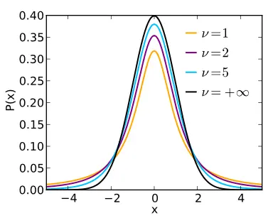
Students t-distribution.

For a coin flip, the sample space is {Heads, Tails} but if you were to sample tree height you’d get a continuous distribution of possible heights. You might be interested in finding the probability of an outcome of some distribution $f(x)$ for all values of $x \leq 4$ (left panel), or for $x = 4$ (right panel).

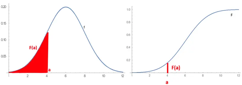
Combined_Cumulative_Distribution_Graphs — Figure 4.
Combinied cumulative distribution graphs.

On the left is the probability density function (pdf) while the right function is the cumulative distribution function (cdf) or integral of $f(x).$ The area in red in the pdf is to the left of $4$ is the value of $F(4)$ in the cdf.

Goldfish and the t-test

Is it true that 40% of goldfish crackers have smiley faces? The only data available are Alan’s count of one package of 349 goldfish. It hardly seems sufficient considering that 142 billion of them are made every year (and it keeps going up!) But, the t-test can give some insight even if we don’t have an exact count.

To determine if the proportion of smiley-faced goldfish crackers in the sample is significantly different from the hypothesized 40%, you can use a one-sample t-test. Here is how to proceed:

State the Hypotheses:

Null Hypothesis ( $𝐻_0$ ): The proportion of smiley-faced crackers in the population is 40%. $𝑝=0.40$ .

Alternative Hypothesis ( $𝐻_1$ ): The proportion of smiley-faced crackers in the population is not 40%. $𝑝 \neq 0.40$ .

Calculate the Sample Proportion:

The sample proportion ( $\hat{p}$ ) is the number of smiley-faced crackers divided by the total number of crackers.

\hat{p} = \frac{142}{349} = 0.4069

Calculate the Standard Error:

The standard error (SE) for the sample proportion is given by:

SE = \sqrt{\frac{p(1-p)}{n}}.

where $p$ is the hypothesized population proportion (0.40), and n is the sample size (349).

SE = \sqrt{ \frac{0.4 \times (1 - 0.4)} {349} } = 0.02622

The Standard Error is a statistic that estimates the amount of uncertainty or error associated with using the sample mean ( $\hat{p}$ ) as an estimate of the true population mean ( $p = 0.4$ ). The standard error shows how much sample means would vary across repeated samples of the same size from the population.

A related concept is the Standard Deviation of the population $\sigma$ . This is a parameter that describes the amount of variability or dispersion in the entire population. It is a fixed unknown quantity that can only be calculated if you have data for the complete population.

The key differences are:

The population standard deviation describes variability in the entire population.
The standard error describes the variability of the sample mean around the population mean.
If the population standard deviation is known, it can be used to calculate the standard error.
If the population standard deviation is unknown, it is estimated by the sample standard deviation (s) when calculating the standard error.

Calculate the Test Statistic:

The test statistic ( $t$ ) is calculated as the difference between the sample proportion and the hypothesized proportion divided by the Standard Error, SE:

t = \frac{ \hat{p} - p}{SE} = \frac{0.4069 - 0.4}{0.02622} = 0.2622

This $t$ value can be compared to the quantiles of a t-distribution with $n-1$ degrees of freedom to determine if the observed difference is statistically significant or not.

A large positive or negative $t$ value indicates the sample proportion deviates significantly from the hypothesized null proportion. A $t$ value close to $0$ indicates the sample proportion is not significantly different from the null hypothesis proportion.

So in essence, this test statistic measures how many standard errors the sample proportion deviates from the null hypothesis proportion. This allows calculating a $p$ -value to decide whether to reject or fail to reject the null hypothesis.

Determine the Degrees of Freedom:

The degrees of freedom (df) is the sample size $p$ minus the number of parameters, $1$ . For this test $𝑑𝑓 =349−1=348.$

Degrees of freedom (df) is a concept in statistics that refers to the number of values or observations in a sample that are free to vary after certain constraints or parameters have been estimated or accounted for.

In the context of the t-distribution and hypothesis testing for a population proportion, the degrees of freedom are equal to $n-1$ , where $n$ is the sample size. Here’s why:

When we calculate the sample proportion $\hat{p}$ from a random sample of size $n$ , we are using all $n$ observations to estimate this one sample statistic. However, once we know the value of $\hat{p}$ and the sample size $n$ , the values of the remaining $n-1$ observations in the sample are not completely “free” - they are constrained by the first observation and the sample size.

More specifically, if we know the sum of $n-1$ observations (call it $S$ ) and the sample size $n$ , then we can calculate the remaining observation as: ( $n \hat{p} - S$ ). So one of the $n$ observations is redundant and does not provide any new information.

Therefore, with $n$ observations used to calculate one sample proportion $\hat{p}$ , we are “using up” 1 degree of freedom, and $n-1$ degrees of freedom remain.

In general, for any statistic calculated from a sample of size $n$ , the degrees of freedom is $n$ minus the number of parameters estimated from the sample data.

Having $n-1$ degrees of freedom allows us to use the appropriate $t$ -distribution percentiles when computing confidence intervals or performing hypothesis tests involving that sample statistic.

Calculate the p-value:

The p-value is the probability of obtaining a test statistic at least as extreme as the one observed, under the null hypothesis. This can be found using the t-distribution with the calculated t-statistic and degrees of freedom.

Using the Omni calculator (one-sample, $\mu \neq \mu_0$ , significance level 0.05) the p-value is $p = 0.7933$ , which is much larger than the significance level of 0.05. Therefore the null hypothesis cannot be rejected, and the proportion of smiley-faced goldfish in the sample is not statistically different from the 40% estimated by The History Channel.

The p-value represents the probability of obtaining a sample proportion as extreme as the one observed ( $\hat{p}$ ), if the null hypothesis about the true population proportion ( $p$ ) is correct.

More specifically:

The null hypothesis specifies a hypothesized value for the population proportion $p$ .
The test statistic $t$ calculates how many standard errors the observed sample proportion $\hat{p}$ deviates from the null hypothesis proportion $p$ .
This test statistic follows a t-distribution with $n-1$ degrees of freedom if the null hypothesis is true.
The p-value is the probability, under the assumption that the null is true, of observing a value of the test statistic at least as extreme as the value actually observed.
A small p-value (typically $\leq$ 0.05 or 0.01) means the sample proportion is very unlikely to have occurred if the null hypothesis proportion is true.
This suggests strong evidence against the null hypothesis, so we reject the null.
A large p-value means the sample data is consistent with what we’d expect if the null were true, so we fail to reject the null.

So in essence, the p-value quantifies how likely or unlikely the sample result is, if we assume the null hypothesis is correct. It helps determine if the data contradicts the null hypothesis significantly.

Significance Levels

Significance levels (denoted by $\alpha$ ) in hypothesis testing are chosen based on the degree of evidence required to reject the null hypothesis. Common choices for the significance level are 0.05 and 0.01, but other values like 0.1 or 0.001 can also be used depending on the situation. Here are some key considerations for choosing the significance level:

Balancing Type I and Type II Errors A lower $\alpha$ reduces the probability of a Type I error (incorrect rejection of a true null hypothesis) but increases the probability of a Type II error (failing to reject a false null). A higher $\alpha$ does the opposite. The significance level essentially controls this trade-off.
Stringency of Evidence Lower values of $\alpha$ like 0.01 require stronger evidence against the null to reject it, making the test more conservative. Higher values like 0.1 are less stringent.
Consequences of Errors In high-stakes scenarios where incorrect rejection is very costly (e.g. judicial contexts), a lower $\alpha$ like 0.01 or 0.001 is preferred. In exploratory studies, a higher $\alpha$ like 0.1 may be acceptable.
Field/Discipline Conventions Many fields have conventional levels, e.g. 0.05 in social sciences, 0.01 in physics. This allows consistency and reproducibility within the discipline.
Number of Tests When multiple tests are performed, lower significance levels help control the overall Type I error rate (e.g. Bonferroni correction).
Sample Size Smaller samples may require higher $\alpha$ to have reasonable power to detect effects. Larger samples allow using lower $\alpha$ .

Ultimately, the significance level is a somewhat arbitrary probability cutoff that is chosen to balance type I/II errors and determine what constitutes statistically significant evidence against the null given the study context and requirements.

A few final thoughts on Student’s t-distribution

Here are a few additional points that could be valuable to know about Student’s t-distribution:

Assumptions The t-distribution assumes the underlying population is normally distributed. Violations of normality, especially with small samples, can affect the validity of the resulting inferences.
Robustness Despite the normality assumption, the t-tests are reasonably robust to departures from normality, especially with larger sample sizes, due to the Central Limit Theorem.
Effect Size While the p-value indicates if a result is statistically significant, the effect size (e.g. Cohen’s d) quantifies the practical/theoretical magnitude of the effect, which is also important to consider.
Confidence Intervals The t-distribution is used to calculate confidence intervals for the population mean when the population standard deviation is unknown.
Relationship to Z-distribution As the sample size increases, the t-distribution approaches the standard normal (Z) distribution. For very large samples, the two are essentially equivalent.
Variations There are variations like the paired/dependent t-test for paired samples, and separate variance t-tests when population variances differ substantially.
Other Applications Beyond one and two-sample t-tests, the t-distribution finds use in regression analysis, ANOVA models, and some nonparametric tests as well.

So in summary, understanding the key assumptions, strengths, limitations, and variations of the t-distribution is important for properly applying and interpreting these widely used statistical tests and procedures.

From Goldfish to Greater Understanding: Why Statistics Matter

A box of goldfish crackers has shown us how statistical tools can help you test claims and draw meaningful conclusions from limited data. Through our analysis of Alan’s careful count of smiley-faced crackers, we demonstrated that:

Even a single sample of 349 crackers could provide meaningful insights when analyzed properly
The observed proportion of 40.69% smiley faces was not statistically different from the claimed 40%
Student’s t-test remains a versatile tool for testing hypotheses

For amateur scientists, statistical testing is important because it:

Provides a systematic way to evaluate claims using limited data
Helps distinguish between meaningful differences and random variation
Allows us to quantify uncertainty in our observations
Enables us to contribute to scientific knowledge even with modest resources

No matter what data you’re collecting, understanding basic statistical concepts helps transform casual observations into meaningful scientific contributions. As Gossett showed through his work at Guinness, sometimes the most practical statistical insights come from everyday questions.

The Goldbach Conjecture

Christian Goldbach sent a letter to fellow Prussian mathematician Leonard Euler (see Seven Bridges for Seven Truckers) on June 7, 1742, in which he said that every even natural number greater than 2 could be expressed as the sum of two prime numbers.

\begin{aligned} 4 &= 2 + 2 \\ 6 &= 3 + 3 \\ 8 &= 3 + 5 \\ 10 &= 3 + 7 \\ &\vdots \end{aligned}

This conjecture remains unsolved but has been verified up to $4 \times 10^{18}$ . The title of this article is a play on The Goldbach Conjecture, something well worth investigating some other time.

Code for this article

A Python JupyterLab notebook is available (goldfish-conjecture.ipynb) to work through these calculations.

Software

JupyterLab - JupyterLab is the latest web-based interactive development environment for notebooks, code, and data.
Python - Python is an interpreted, high-level and general-purpose programming language.

Image credits

Hero: How to Take Care of Goldfish, petMD
Goldfish crackers: Wikipedia Goldfish (cracker)
William Sealy Gosset: [Wikipedia](By User Wujaszek on pl.wikipedia - scanned from Gosset’s obituary in Annals of Eugenics, Public Domain, https://commons.wikimedia.org/w/index.php?curid=1173662)
Student t-distribution: Wikimedia Commons, Skbkekas
Combined Cumulative Distribution Graphs: Wikimedia Commons ShristiV