The Big Squish Theory - Part II
Models, Mangles and Meshes
Ask NotebookLMBaubles, bangles, hear how they jing, jinga-linga
Baubles, bangles, bright shiny beads
Sparkles, spangles, her heart will sing, singa-linga
Wearin’ baubles, bangles and beads
- “Baubles, bangles and beads” from the musical Kismet, sung by Frank Sinatra
Computational Fluid Dynamics
Computational Fluid Dynamics (CFD) is used to model the motion of fluids. A volume of fluid is decomposed into many small cells where the physical properties of each cell can be calculated. The effects of actions on one cell are propagated to adjacent cells to determine the fluid flow. A numeric CFD solver can calculate pressures, temperatures, and fluid flows within a volume over very short time steps.
Recall from the previous post, The Big Squish Theory - Part I, that we tried to solve the Euler equations using the Wolfram Language, but found that the equations were too stiff.
Numerical solvers are often better able to handle stiff CFD problems. To solve the Euler equations numerically, we first need to create a grid, or stencil. In one direction are the steps in spatial dimension, , and the other direction are the time steps, .
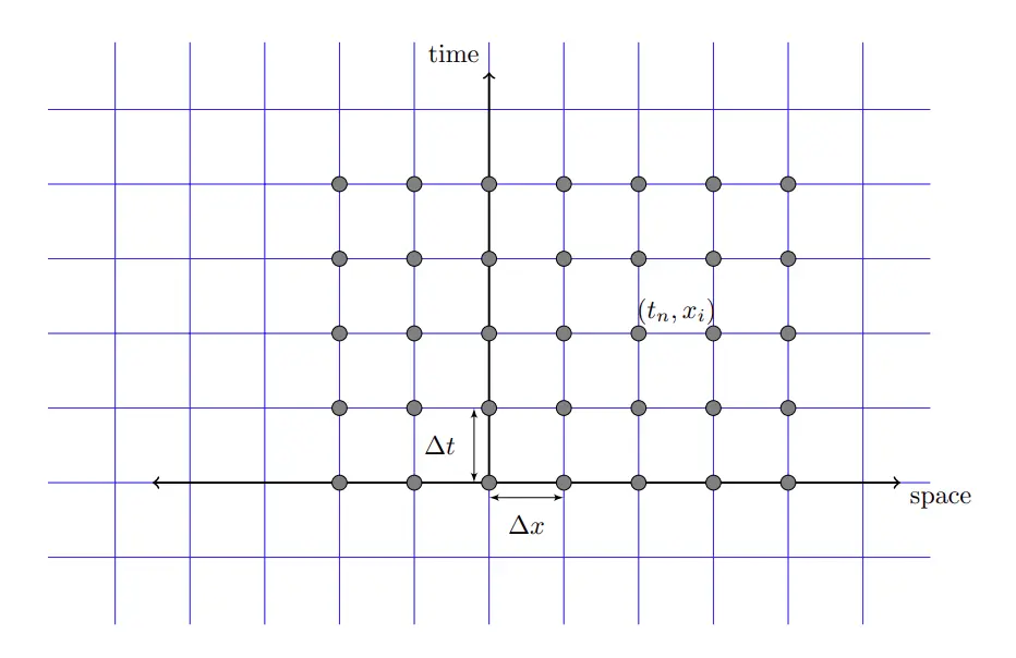
CFD stencil.
Usually, numerical schemes calculate conditions by looking at the effects of nearby points in followed one by a time step forward. PDE solvers typically use a method-of-lines approach. This semi-discretizes the spatial derivatives, converting the PDE into a system of ODEs in time.
An appropriate time step size is then chosen to numerically integrate this ODE system, often using stability criteria like the Courant-Friedrichs-Lewy (CFL) condition,
where is the Courant number, and is the maximum velocity of the problem. The Courant number is a dimensionless number that measures how fast the solution is changing in space compared to how fast it is changing in time. A smaller Courant number means that the solution is changing more slowly in space, and therefore a larger time step can be used.
The time step in Euler’s is the left term
Computers work in discrete increments, so rather than calculating the instantaneous slope of each of these parameters we’ll have to use a small time step . Many methods for solving partial differential equations (PDEs) estimate conditions at several intermediate time steps and then combine the answers for conditions at the next time step.
We will also need to update conditions from nearby points using the second term
that defines the rate of change of density, velocity, and specific energy. The spatial dimension is updated first because the fluxes, or changes in these parameters at the edges of the region depend on the solution at the current time step.
Once the spatial step has been chosen, the CFL condition can be used to calculate the maximum time step. The time step must be less than or equal to the maximum time step to ensure stability of the numerical solution.
In some cases, it may be necessary to use a smaller time step than the maximum time step to achieve the desired accuracy of the solution. This is often the case for problems with sharp features, such as shock waves.
Numerical solvers generally handle the time step part of the stencil but require the spatial coordinates as an input. For this, we need a way to build a model in 1,2, or 3 dimensions and a way to create a mesh on the model.
Models
Model Equations
Before you build the model, you should think about what problem you’re trying to solve and the PDE (partial differential equation) required. Some PDEs that can be solved on meshes are:
- The Laplace equation - describes the equilibrium of a scalar field. It is often used in modeling problems involving heat transfer, electrostatics, and fluid flow.
- The Poisson equation - similar to the Laplace equation, but it also includes a source term. This source term can be used to model things like point charges or heat sources.
- The Navier-Stokes equations - describe the motion of fluids. They are the most important equations in fluid dynamics and are used in a wide variety of applications, such as modeling the flow of air around an airplane or the flow of blood through an artery.
- The Maxwell equations - describe the behavior of electromagnetic fields. They are used in a wide variety of applications, such as modeling the behavior of antennas or the propagation of light.
- The Schrödinger equation - describes the behavior of quantum particles. It is used in a wide variety of applications, such as modeling the behavior of electrons in atoms or the behavior of photons.
- The Klein-Gordon equation - similar to the Schrödinger equation, but it is used to describe the behavior of massive particles.
- The Dirac equation - describes the behavior of relativistic particles.
- The Burgers equation - describes the evolution of a one-dimensional wave. It is often used as a model for traffic flow.
- The Korteweg-de Vries equation - describes the evolution of a one-dimensional wave with dispersion. It is often used as a model for shallow water waves.
- The Navier-Stokes-Korteweg equations - describes the motion of a fluid with surface tension. They are used in a wide variety of applications, such as modeling the behavior of soap films or the behavior of droplets.
- The Cahn-Hilliard equation - describes the evolution of a two-phase system. It is often used as a model for phase separation or for modeling the behavior of fluids with surfactants.
Coupling the heat equation with Navier-Stokes allows you to model flows of heated fluids. Some applications of PDE solvers are
- Acoustics
- Electromagnetism
- Heat transfer
- Fluid dynamics
- Material science
- Structural mechanics
- Biomedical engineering
Constructive Solid Geometry
Constructive Solid Geometry (CSG) is a technique used in solid modeling to represent solid 3D objects using Boolean operations on primitive shapes. Usually, the basic shapes consist of cubes, spheres, cylinders, and polyhedra combined using union, intersection, and difference operations. The Boolean operations are:
- Union : Joins two solid objects into one aggregated object.
- Intersection : Keeps only the area or volume common to two objects.
- Difference : Subtracts one object from another.
An example is this object derived from three cylinders, a cube, and a sphere:
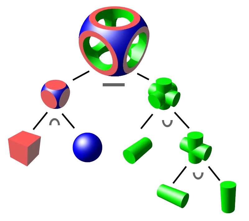
Constructive solid geometry union and differences of a cube, sphere and cylinders.
CSG provides an intuitive way to model complex shapes using simple operations. Models are editable and parametric, but some shapes are difficult to represent. CSG models have trouble representing freeform sculpted surfaces.
A good place to get started with CSG is with OpenSCAD. The commands to build objects are pretty intuitive, so let’s try making the object shown above. The outline is called a tree, and the primitive objects at the ends of branches are called leaves.
On the left, two primitive objects, the cube and the sphere, are combined using an intersection operation to build the node above them. On the right, three cylinders are combined with a union operator after rotation to new orientations. Finally, taking the difference between the two new objects creates the finished form.
The OpenSCAD cheat sheet shows all of the possible basic shapes in 2D and 3D, as well as the Boolean operations, and possible transformations. A good way to get started is to build the cube on the left with: cube([1, 1, 1], center = true);. The dimensions are contained in the vector , and the command center = true puts the center of the cube at the origin. Note the semicolon at the end of the line. Press F5 to display the cube.
Since each side is length , then the distance from the center to the middle of any side is , and the distance from the center to each corner is . If the radius of the sphere is less than then the intersection with the cube leaves just the sphere, while if the radius is greater than the intersection leaves only the cube.
Spheres are automatically centered at the origin, and the command $fn=128 sets the number of facets used to represent the sphere since OpenSCAD can’t perfectly generate smooth rounded surfaces.
Here is the complete code to create the model.
// Shape parameters
sphereRadius = 0.65;
cylinderRadius = 0.3;
cylinderHeight = 1.1;

// Top-level difference operation
difference(){

    // Intersection of cube and sphere
    intersection(){

        // Red cube with unit sides
        color("red", 1.0){
            cube([1, 1, 1], center = true);
            }

        // Blue sphere
        color("blue", 1){
            sphere(r = sphereRadius, $fn = 128);
            }
        }

    // Union of three cylinders centered on each axis
    color("Lime", 1.0){
        union(){
            union(){
                cylinder(h = cylinderHeight, r = cylinderRadius, $fn = 128, center = true);
                rotate([90,0,0]){
                cylinder(h = cylinderHeight, r = cylinderRadius, $fn = 128, center = true);
                }
            }
            rotate([0,90,0]){
                cylinder(h = cylinderHeight, r = cylinderRadius, $fn = 128, center = true);
            }
        }
    }
}
The rendered model looks like this:
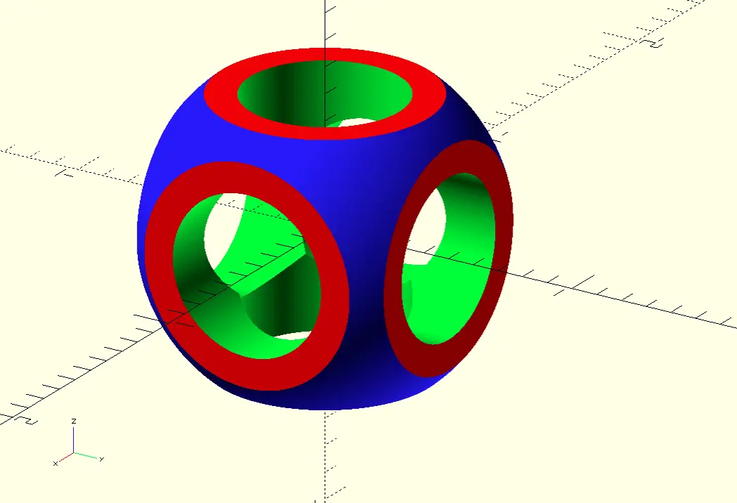
OpenSCAD model.
Other CAD (computer-aided design) systems can perform parametric modeling using Boolean logic on shapes, such as Open Cascade Technology (OCCT), FreeCAD, and Salome.
Mangles
Before we get into the details of mesh construction, there are times when the code used to construct the mesh creates an imperfect mesh. This can happen if the edges of adjacent cells don’t line up together, or if more than two faces connect to the same edge.
Fixing these problems can be tricky, and you’ll need software tools designed for these issues. Meshlab is very good at correcting mangled meshes, but may take a while to learn how to best fix the problems. For the BST the layout is simple so we won’t encounter any issues with the mesh. If the mesh is error-free, it is said to be “watertight”.
Meshes
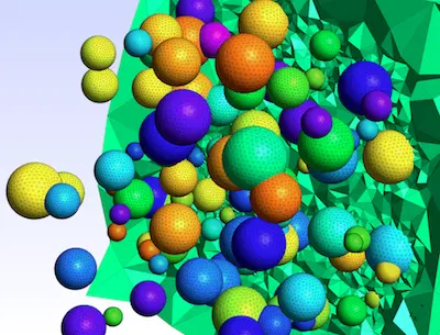
Most meshes are formed from triangles or tetrahedra. A typical mesh looks like this,
CSG mesh.
but for the BST problem, we only need to slice the box along the length to form a series of thin cells.
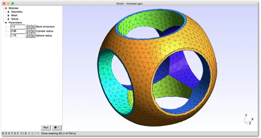
GMSH
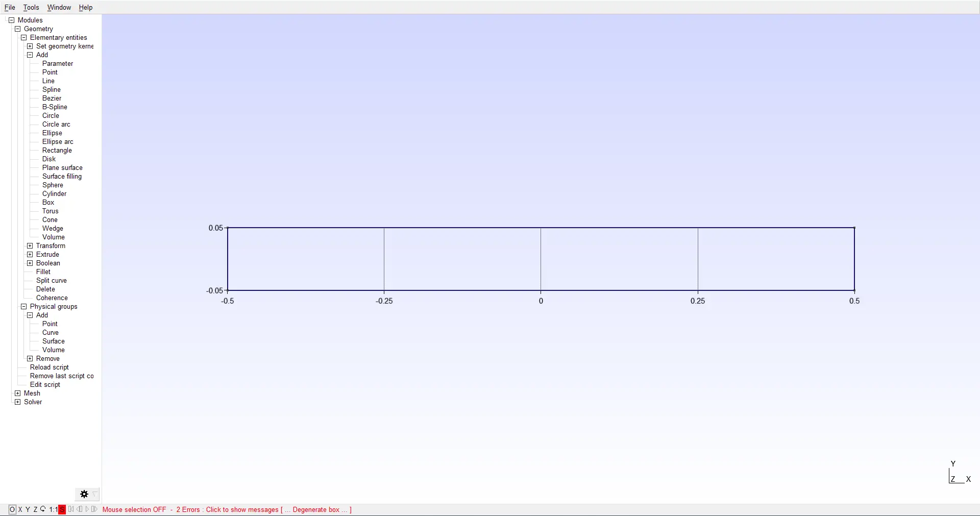
Gmsh is a two or three-dimensional finite element mesh generator using Open Cascade Technology to generate models with constructive solid geometry. Download and install the latest version, and start Gmsh. For the Big Squish Theory simulation, any dimensions will do, but for the image below the dimensions are for the location and for and .
Gmsh shock tube.
To create each cell, we need to define the four vertices or points at the corners of the rectangle. Next, connect each pair of adjacent points with lines, then define a Line Loop that outlines the rectangle, and finally call the Line Loop a Surface.
Gmsh has a reserved term, Transfinite, which in mathematics means going beyond or surpassing any finite number, group, or magnitude. For Gmsh, this means that you can create or position lines, curves, surfaces, and volumes with non-integer values.
It sounds confusing, but it means that you can tell Gmsh that you want cells along the length of the rectangle, and it will figure out where to put the lines separating the cells, even if the locations are non-integer positions.
In Gmsh, the code to create the 2D shock tube for the Big Squish Theory is:
// Gmsh project created on Mon Jun 17, 2024
SetFactory("OpenCASCADE");

// Define points
L = 0.5;    // Tube length
H = 0.05;   // Tube width
N = 10;     // Number of rectangles along length of the tube
Point(1) = {0, 0, 0, 1.0};
Point(2) = {L, 0, 0, 1.0};
Point(3) = {L, H, 0, 1.0};
Point(4) = {0, H, 0, 1.0};

// Connect points with lines to form the rectangle
Line(1) = {1, 2};
Line(2) = {2, 3};
Line(3) = {3, 4};
Line(4) = {4, 1};

// Define the rectangle as a surface
Line Loop(5) = {1, 2, 3, 4};
Plane Surface(6) = {5};

// Define transfinite lines with a specific number of nodes
Transfinite Line {1,3} = N+1; // Adjust number for refinement in length of the tube
Transfinite Line {2,4} = 1;   // Adjust number for refinement in the width of the tube

// Define transfinite surface using the specified lines
Transfinite Surface {6} = {1,2,3,4};

// Recombine the surface mesh into quadrilaterals
Recombine Surface {6};

// Set the mesh element size
Mesh.CharacteristicLengthMax = 0.1;

// Generate the 2D mesh
Mesh 2;

// Save the mesh to a file
Save "shock_tube.msh";
In Gmsh click File Open and select the file shock_tube.msh to view the mesh. A handy editor for Gmsh files is Notepad++.
Mesh Formats
Meshes come in many formats. We’ll give links to some of the standard formats, and show how to create a mesh from the locations of the vertices and the list of vertex links. Common mesh formats are:
- brep - a method for representing a 3D shape by defining the limits of its volume. A solid is represented as a collection of connected surface elements, which define the boundary between interior and exterior points. Developed by OpenCascade Technology.
- step - a widely used exchange form of STEP. ISO 10303 can represent 3D objects in computer-aided design (CAD) and related information. Due to its ASCII structure, a STEP file is easy to read, with typically one instance per line.
- mesh - three-dimensional models composed of points, lines, and faces that allow for the creation of 3D objects and environments.
- cgns - CFD General Notation System (cgns). It is a general, portable, and extensible standard for the storage and retrieval of CFD analysis data. It consists of a collection of conventions, and free and open software implementing those conventions.
- off - a geometry definition file format containing the description of the composing polygons of a geometric object. It can store 2D or 3D objects, and simple extensions allow it to represent higher-dimensional objects as well.
- stl - Stereolithography (stl) is a file format native to the stereolithography CAD software created by 3D Systems.
- vtk - The Visualization Toolkit provides several source and writer objects to read and write popular data file formats. The Visualization Toolkit also provides some of its own file formats. The main reason for creating yet another data file format is to offer a consistent data representation scheme for a variety of data set types and to provide a simple method to communicate data between software.
- ply - the Polygon File Format or the Stanford Triangle Format is designed to store three-dimensional data from 3D scanners. The data storage format supports a relatively simple description of a single object as a list of nominally flat polygons.
- su2 - SU2 mainly uses a native mesh file format as input into the various suite components. Limited support for the CGNS data format has also been included as an input mesh format. The code, SU2, is a suite of open-source software tools written in C++ for the numerical solution of partial differential equations (PDE) and performing PDE-constrained optimization.
Now go have some beer, bangers and mash. Next time we’ll run the Big Squish Theory simulation in SU2.
Bangers and Mash.
Code for this article
- OpenSCAD model, CSG_example.scad
- Gmsh shock tube, shock_tube.geo
Software
- gmsh - Gmsh is an open source 3D finite element mesh generator with a built-in CAD engine and post-processor.
- SU2 - SU2 is a suite of open-source software tools written in C++ for the numerical solution of partial differential equations (PDE) and performing PDE-constrained optimization.
- OpenSCAD - OpenSCAD is software for creating solid 3D CAD models using constructive solid geometry and extrusion of 2D outlines.
- Notepad++ - Notepad++ is a free (as in “free speech” and also as in “free beer”) source code editor and Notepad replacement that supports several languages.
- Meshlab - Meshlab, the open source system for processing and editing 3D triangular meshes.
Image credits
- Hero: Gmsh, A three-dimensional finite element mesh generator with built-in pre- and post-processing facilities. Christophe Geuzaine and Jean-François Remacle.
- CFD Stencil: CFD Julia: A Learning Module Structuring an Introductory Course on Computational Fluid Dynamics, Suraj Pawar and Omer San, MDPI 2019.
- Constructive Solid Geometry: Wikimedia Commons, CSG tree, Created and rendered in POV-Ray.
- Gmsh Shock Tube: Gmsh.
- OpenSCAD model: OpenSCAD, The Programmers Solid 3D CAD Modeller.
- CSG Mesh: New CAD features, Gmsh 3.0 and API, C. Geuzaine, Third Gmsh Workshop, Lanzarote, March 29-31, 2017.
- Bangers and Mash: Irish Bangers and Colcannon Mash, The Original Dish, March 13, 2021.