

Extending Time
Cesàro Sums, String Theory, and Vantablack in 3D!
Ask NotebookLMHe say, “One and one and one is three”
Got to be good-lookin’ ‘cause he’s so hard to see
- Come Together, The Beatles
The Face of Time
For my birthday this year, Sara and Max gave me a math clock with the hours shown as trigonometric identities. Time is a concept we encounter every day, often represented by the simple numbers 1 through 12 on a clock face.
But what if we could reimagine these numbers, expressing them with the most esoteric formulas I could think of? Well, they could be worse, but I didn’t want the formulas to get too large. This article looks into some unusual mathematics, from Euler’s Identity to Cesàro summability, and even touches on the interesting connections to string theory.
The next idea I had was to 3D print the equations onto disks that could be clipped to the edge of the clock so I could have both versions. The original angle versions would still be visible, but the new equations could be extended around the edges.
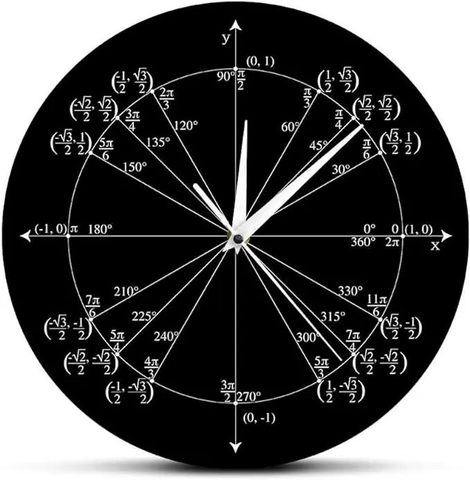
The math clock.
We’ll explore the world of mathematical expressions, from simple arithmetic to complex theories, and discover alternative ways to represent the numbers on a clock face. The first step was to come up with unique expressions for the numbers 1 through 12, and along the way, we’ll dive into Cesàro summability, string theory, and 3D printing.
So here are the formulas for each hour of the clock.
One
and is considered the most beautiful equation in mathematics because it combines the exponential function , the imaginary number , the ratio of the circumference of a circle to its diameter, and the additive and multiplicative identities and .
Geometrically, the complex number is a point in the complex plane with coordinates . It can also be thought of in terms of polar coordinates, where and is the counterclockwise angle from the axis.
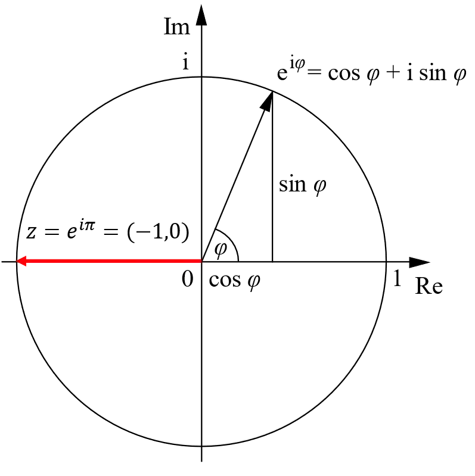
Euler’s identity in the complex plane.
Euler’s formula says that and when , is the point so .
Two
In base 2, . It just looks like it was put on the wrong side of the clock.
Three
If are in arithmetic progression then
An arithmetic progression is a sequence of integers such that the differences between any two successive terms remain the same. The sequence is an arithmetic progression because the difference between the numbers is always .
Let be the constant between successive terms of an arithmetic sequence, . Then, write the expression above in terms of , and use the fact that the difference of squares is
to get the result.
Four
Five
This is just a rearrangement of the Golden ratio
Six
Six is .
Seven
This is an approximation:
To get this approximation, let’s evaluate the sum inside the parentheses: . This series can be derived from the geometric series
Differentiating both sides with respect to ,
and then multiplying both sides by ,
The term can be omitted since The value of here doesn’t matter so long as . Letting gives
Substitute this back into the original expression to get
Eight
We’ll combine eight and nine, so , and
Nine
.
Ten
The term in the middle is , and everything else is the integral of the normal distribution which by definition must be . The second line is a bit more compact.
Eleven
In base , eleven is . We probably should have written , but it would have taken away some of the obfuscation.
Twelve
For the equation at high noon, we’ll use the fact that the infinite sum,
This sum looks completely impossible, but it depends on a special interpretation of the sums of infinite sequences and leads to an important result in string theory.
Ernesto Cesàro was an Italian mathematician who worked mainly in the area of differential geometry.
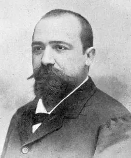
Ernesto Cesàro
He thought about infinite series, and how you might define the sum of such a series even if it doesn’t converge. In Seven we used the convergent geometric series to derive the approximation, but not all series converge which means that the infinite sum doesn’t approach a finite value. There are several tests to determine whether an infinite series is convergent or divergent.
Cesàro thought about series that are somewhere between convergent and divergent. Maybe the series doesn’t settle down to a single value, but what if the average does? For example, the series has partial sums (sums after the first terms) of . Cesàro saw that the average does converge because the sum of this new sequence divided by the number of terms becomes
Another way to think about this is to let be the sum The terms may be grouped in two ways,
Adding the two rows together gives or . So the question Cesàro asked was, does the sum converge to , or nothing at all?
Let’s carry on with the Cesàro sum of and let be the series
Now, add , but with the second shifted by one place,
so or .
Now define a new series
and take the difference between and ,
Thus so
Now high noon can be expressed as
This seems like the mathematical weirdness equivalent of quantum mechanics! In fact, this strange identity is used in string theory to combine the ideas of general relativity and quantum mechanics.
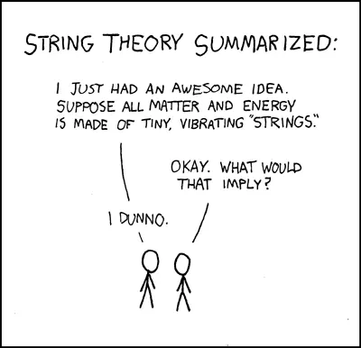
String Theory
Physics has two main branches of thought - general relativity and quantum mechanics, and string theory attempts to reconcile the two. General relativity gives a geometric interpretation of gravity in which space and time are deformed by mass.
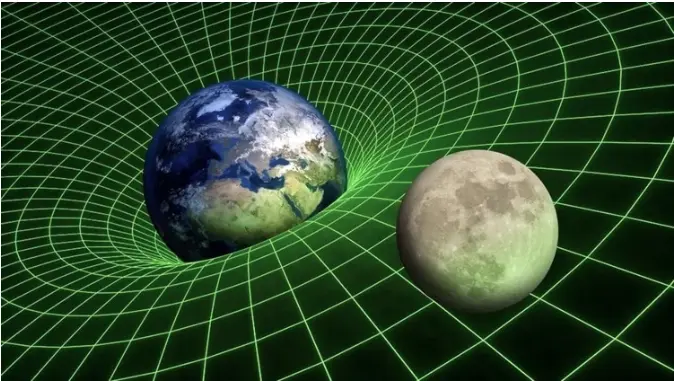
Spacetime warping.
General relativity has been thoroughly tested and shown to explain the slight perturbation of Mercury’s orbit due to the mass of the Sun, and how the speed of light is reduced in the presence of a large mass.
While general relativity operates mainly on very large scales, quantum mechanics is valid for small scales, mainly at the size of atoms and below.
Quantum mechanics is the branch of physics that deals with the behavior of matter and energy at the smallest scales, such as atoms and subatomic particles. It introduces concepts that differ significantly from classical physics, including wave-particle duality, quantization of energy levels, and the principle of superposition, where particles can exist in multiple states simultaneously until measured.
Quantum mechanics successfully describes three of the four fundamental forces of nature—electromagnetism, the strong nuclear force, and the weak nuclear force—through the framework of quantum field theory.
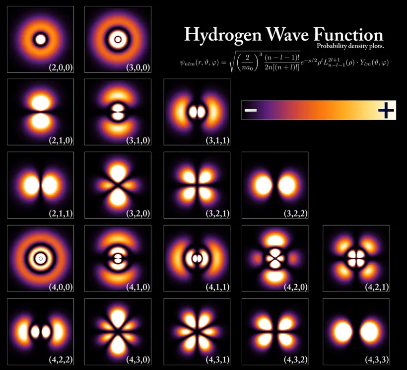
The hydrogen wave function.
The Gravity Problem
The challenge arises when trying to incorporate gravity into this quantum framework. Gravity is described by general relativity, formulated by Albert Einstein, which portrays gravity not as a force but as the curvature of spacetime caused by mass. In this view, massive objects like planets and stars warp the fabric of spacetime, and other objects move along the paths dictated by this curvature. This geometric interpretation contrasts sharply with the particle-based approach of quantum mechanics, where forces are mediated by particles (like photons for electromagnetism).
The fundamental incompatibility stems from the fact that general relativity operates in a smooth, continuous spacetime, while quantum mechanics relies on discrete, quantized interactions. When physicists attempt to apply quantum principles to gravity, they encounter significant difficulties, such as non-renormalizable infinities that arise in calculations involving gravitational interactions. This means that, unlike the other forces, gravity does not fit neatly into the quantum framework, leading to the so-called “gravity problem.”
Efforts to unify quantum mechanics and general relativity into a single coherent theory, often referred to as quantum gravity, have led to various approaches, including string theory and loop quantum gravity. However, a complete and experimentally validated theory that successfully merges these two foundational pillars of physics remains elusive. The quest for such a unifying theory continues to be one of the most profound challenges in modern theoretical physics.
String theory as a solution to the gravity problem
String theory is a theoretical framework in physics that attempts to reconcile quantum mechanics and general relativity. String theory says that the fundamental constituents of the universe are not point-like particles, but rather tiny, vibrating strings of energy. These strings, which exist in multiple dimensions beyond the four we can observe (three spatial and one time), vibrate in different ways to give rise to all the particles and forces we see in nature.
The idea of string theory first arose in the late 1960s and has since evolved into a complex and multifaceted field of study. One of its most striking features is the assertion that our universe may have many more dimensions than we can perceive – typically 9, 10, or 25 dimensions of space. These extra dimensions are thought to be compactified, or curled up so tightly that they are invisible to us, yet they play a crucial role in determining the properties of our universe (see C is for Calabi-Yau Manifolds).
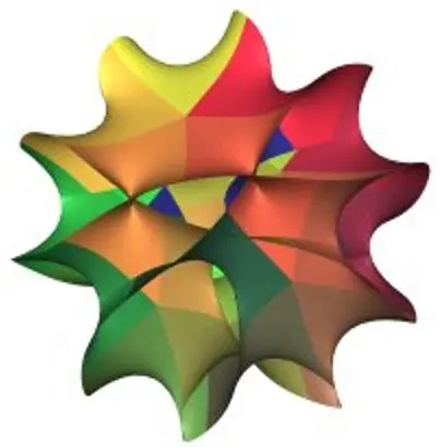
Calabi-Yau manifold.
String theory has the potential to unify all fundamental forces and particles under a single theoretical umbrella and it offers a way to describe gravity at the quantum level, but it remains highly speculative. It has yet to make testable predictions that could conclusively prove or disprove its validity, leading to ongoing debates about its place in modern physics. Nonetheless, the mathematical insights derived from string theory have had far-reaching impacts in various areas of theoretical physics and mathematics, ensuring its continued relevance in scientific discourse.
String theory, a theoretical framework in which the point-like particles of particle physics are replaced by one-dimensional objects called strings, has a profound relationship with Cesàro sums. In the context of string theory, Cesàro sums are often used to deal with the infinities that arise in the calculation of the energy levels of a string. The energy levels of a string are given by a series that is divergent, meaning that it does not have a finite sum in the usual sense. However, by using Cesàro summation, one can assign a finite value to this series. This finite value is then interpreted as the physical energy of the string.
Moreover, the use of Cesàro sums in string theory is not just a mathematical trick but has deep physical implications. It is related to the fact that string theory includes a new kind of symmetry, called “worldsheet duality”, which is not present in ordinary particle physics. This symmetry essentially states that a string propagating in a space with a large radius of curvature is equivalent to a string propagating in a space with a small radius of curvature. The use of Cesàro sums is crucial for this duality to hold.
Cesàro sums are an essential tool in string theory, used to make sense of the divergent series that appear in the theory and to ensure the consistency of the theory’s novel symmetries.
Cesàro sums in String Theory
The infinite sum resulting from Cesàro summation is a result that arises from the realm of analytic continuation and regularization techniques in mathematics. This result, while counterintuitive, finds significant applications in string theory, particularly in the context of quantum field theory and the calculation of certain physical quantities.
In string theory, the concept of a string propagating through spacetime leads to the emergence of various mathematical structures, including the need to handle infinite sums. The sum can be interpreted through the lens of zeta function regularization, where the Riemann zeta function is analytically continued to values where it does not converge. This result is crucial in string theory, particularly in the calculation of the vacuum energy of strings. When considering the quantum fluctuations of strings, one encounters divergent sums that can be regularized using this technique. The negative value of can be interpreted as a contribution to the energy density of the vacuum, which has profound implications for the stability and dynamics of string theory models.
The application of this sum in string theory is not merely mathematical; it has physical consequences. For instance, the appearance of in calculations related to the Casimir effect—a phenomenon where vacuum fluctuations lead to observable forces between objects—demonstrates how such infinite sums can influence physical predictions. In string theory, the regularization of these sums allows physicists to derive finite results from otherwise divergent series, leading to a more coherent understanding of the underlying physics. In summary, the infinite sum serves as a powerful tool in string theory, enabling the treatment of divergences and contributing to the rich tapestry of quantum field theory. Its implications extend beyond mathematics, influencing our understanding of fundamental forces and the structure of the universe.
The Casimir Effect
The Casimir effect is a physical phenomenon that arises from the quantum fluctuations of the vacuum between two closely spaced conductive plates. When these plates are placed in a vacuum, they restrict the types of virtual particles that can exist between them, leading to a measurable force that pulls the plates together. This effect is a direct consequence of quantum field theory, where the vacuum is not empty but filled with fluctuating fields.
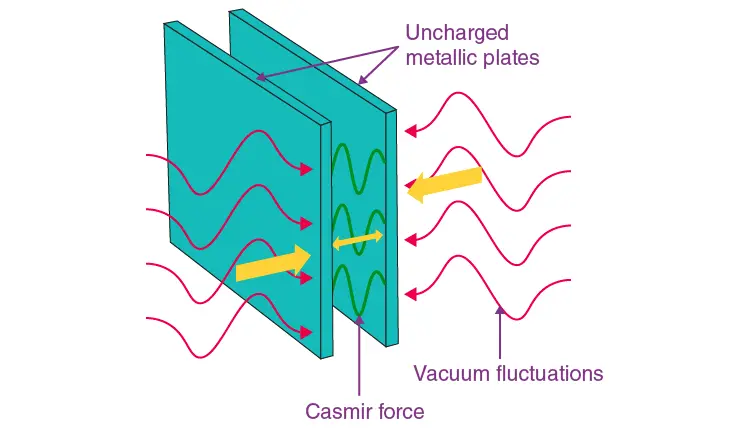
The Casimir effect.
The energy density of these fluctuations can be calculated by considering the allowed modes of oscillation between the plates, which leads to an infinite sum over the frequencies of these modes.
To compute the energy associated with these modes, one typically encounters divergent sums. For instance, the energy density can be expressed as:
where is the separation between the plates. This sum diverges, but through the technique of zeta function regularization, one can assign a finite value to it. This is where the Riemann zeta function comes into play.
Riemann Zeta Function and Regularization
The Riemann zeta function, , is defined for complex numbers with a real part greater than as:
However, it can be analytically continued to other values of , including negative integers. For example, at , the zeta function yields:
This result is particularly striking because it implies that the sum of all natural numbers, , can be assigned the value through this regularization process.
In the context of the Casimir effect, the energy density can be expressed in terms of the zeta function, allowing physicists to extract meaningful physical predictions from otherwise divergent series. The regularization effectively “removes” the infinities by subtracting divergent contributions, leading to a finite and physically significant result.
The relationship between the infinite sum of natural numbers and the Riemann zeta function is rooted in the concept of analytic continuation. While the series diverges in the traditional sense, the zeta function provides a framework to assign it a finite value through a process that involves complex analysis. This connection illustrates how mathematical techniques can bridge the gap between abstract mathematics and physical phenomena, such as the Casimir effect, where the implications of these sums manifest in observable forces and energies in quantum field theory.
In summary, the Casimir effect demonstrates the utility of the Riemann zeta function in regularizing divergent sums, allowing physicists to derive finite results from infinite series, thereby enhancing our understanding of quantum mechanics and field theory.
But, before we get too excited about the future of string theory, Peter Woit writes in his review of Joseph Conlon’s book Why String Theory?
Of the fourteen chapters of the book, chapter 7 is entitled “Direct Experimental Evidence for String Theory.” Here’s the entire content of chapter 7:
There is no direct experimental evidence for string theory.
Maybe physicists should rethink zeta function regularization?
FreeCAD
With that diversion into string theory, let’s get back to 3D printing mathematics.
To build the 3D-printed parts for the equations, I chose FreeCAD, an open-source parametric computer-aided design system. Start FreeCAD, and select the Part workbench. Choose the top view so the axis points to the right and the axis is up. The clip is composed of cubes, cylinders, and a ring fused with Boolean operations.
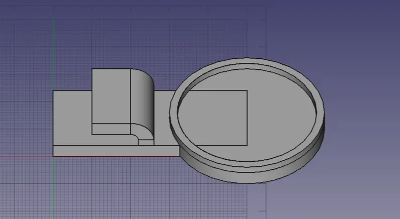
Equation clip in FreeCAD.
To generate the equation images, I used the online Equation Editor and downloaded the image in .svg format, 20-point font, 120-pixel output resolution with transparent background and block compression. To make the equation bold, put the LaTeX in math bold, e.g. \mathbf{10}. Another option is to use the LaTeX Previewer using $$ \mathbf{14_7} $$.
Import the .svg figure into TinkerCAD and adjust the dimensions. You can adjust the length and width by dragging a corner to a new position. Record the dimensions before making the adjustments so you can maintain the ratios. After adjusting the length and width, use the pop-up dialog to set the height to 4 mm.
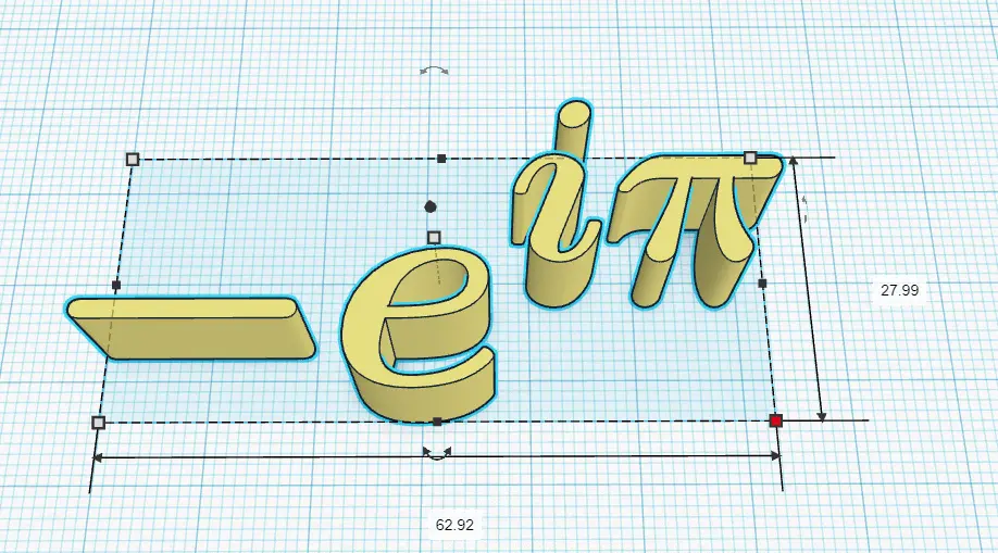
Euler’s Identity in TinkerCAD.
I thought it might be fun to paint the clip with Vantablack, a paint that absorbs over 99% of incident light and has got to be good-lookin’ ‘cause it’s so hard to see. Rolling orange paint onto the equations would make them appear to float over an abyss of nothingness. I assume that Vanta Black is the antimatter nemesis of Vanna White.
*See: 3D Print SVG Lineart (Inkscape and Tinkercad) *
Equation clip dimensions
How big can we make the clips? This question was posed in the Classical Mathematics Group, what is the ratio of to ?
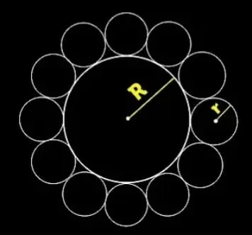
Circle ratios.
The ratio
so to simplify the notation, let . Then
Since and
when , and for
With that, you have all of the tools to either extend time or waste time. Your choice.
Software
- FreeCAD - FreeCAD is an open-source parametric 3D modeler made primarily to design real-life objects of any size.
References and further reading
- What is String Theory? Brian Greene, World Science Festival, Jul 25, 2019
- What is string theory? Nick Geiser, Space.com, May 18, 2023
- String Theory, NewScientist
- String Theory, Byju’s
- Why Is M-Theory the Leading Candidate for Theory of Everything? Natalie Wolchover, Quanta Dec 18, 2017.
- String Theory For Dummies Cheat Sheet, Andrew Zimmerman Jones and Alessandro Sfrondrini, Jun 30, 2022.
- String theory: it’s not dead yet. Sean Carroll, NewScientist, May 19, 2007.
- String Theory Ties Us in Knots, ABC Science, Aug 31, 2010.
- The roots and fruits of string theory. Matthew Chalmers, CERN Courier, Oct 29, 2018.
- Understanding vacuum fluctuations in space, University of Regensburg Aug 10, 2020.
- C is for Calabi-Yau Manifolds, Andreas Braun
- The Most Astonishing Proof In String Theory: How The Sum 1+2+3+4+… Is Equal To -1/12?, Akash Peshin, Oct 19, 2023.
- Two physicists explain: The sum of all positive integers equals −1/12. Steven T. Corneliussen, Feb 4, 2014.
- What do we get if we sum all the natural numbers?. Tony Padilla.
- The Euler-Maclaurin formula, Bernoulli numbers, the zeta function, and real-variable analytic continuation. Terence Tao, Apr 10, 2010.
- Divergent Series: why 1+2+3+··· = −1/12. Bryden Cais.
- The Paradox of 1 – 1 + 1 – 1 + 1 – 1 + … Jack Murtaugh, Scientific American, Aug 16, 2024
- Why Einstein’s General Relativity Theory Is Still Right After 100 Years, Robert Lea, AZO Quantum, Aug 8, 2022.
- Relativity’s Long String of Successful Predictions, Adam Hadhazy, Discover Magazine, Feb 25, 2015.
- What is the theory of general relativity?. Nola Taylor Tillman, Meghan Bartels, Scott Dutfield, Space.com, May 14, 2023.
- DOE Explains…Quantum Mechanics, DOE Office of Science.
- The Physicist Who’s Challenging the Quantum Orthodoxy.
- Is Space Pixelated? Whitney Clavin, Caltech Magazine, Nov 29, 2021.
- Science and technology of the Casimir effect, Alexander Stange; David K. Campbell; David J. Bishop, Physics Today, Jan 2021
Image credits
- Hero: The Persistence of Memory, Salvador Dali, 1931.
- One: Wikimedia Commons - Gunther
- Ernesto Cesàro: Wikimedia Commons
- Spacetime Warping: canbedone/Shutterstock
- The Hydrogen Wave Function: DOE Explains…Quantum Mechanics
- Calabi-Yau Manifold: C is for Calabi-Yau Manifolds
- Casimir Effect: BYJU’s
- String Theory Summarized: XKCD, Randall Munroe
- Equation clip in FreeCAD
- Euler’s Identity in TinkerCAD
- Circle Ratios: Classical Mathematics Group