
The Hormuz Closure - What Standard Analysis Misses
A System Dynamics Model of Compounding Feedbacks
Ask NotebookLMAt the time of this writing, the conflict in the Middle East is ongoing, and the full impact of the Hormuz closure is not yet known. However, it is clear that the closure has had a major impact on the flow of goods around the world. Others are weighing in on the topic, providing their analysis and insights. Here are some of them:
- Don’t Look Up! - What previous oil crises can teach us about this one, and what to expect in 2027 and beyond
- The Persian Polycrisis - What can we do now, that the damage has been done?
- The Myth of American Energy Independence - Make America Drained Again
- There Is No “Next Economy”. If we ruin this one, well, then that was it
- The Right Side of Chaos
- Game of Drones: The New World Disorder
- America Has Plenty of Oil — Just Not the Right Kind
- How is this possible? Seriously.
- By Hideaway: Drill Steel – One of many Iran war CACTUS triggers
- Why Isn’t Oil Above $200 Yet?
- The Logic of NACHO
- ‘Not a Chance Hormuz Opens’: How Wall Street’s new NACHO trade bets on a prolonged oil shock
Abstract
The February 2026 Hormuz closure is analyzed through neoclassical and biophysical economics views. The neoclassical model says that a price signal generates a supply response, and equilibrium is restored. We argue this framing misses three physical mechanisms that compound and are only partially irreversible, a view more in line with biophysical economics. Crude quality mismatch makes shale a structurally inadequate substitute, a sulfur-nitrogen chain simultaneously constrains critical mineral extraction and food production, and reservoir neglect permanently damages Gulf capacity after 3–5 years without investment. We present a System Dynamics model (8 stocks, 11 flows, 39 auxiliaries) calibrated against IEA data and historical oil shocks. The model incorporates Garrett’s thermodynamic GDP-energy coupling and geologically-inferred reserve estimates. Six closure-duration scenarios (2 months to 5 years) demonstrate that the open question is not whether there will be lasting damage, but how much, and that depends on the closure duration.
Introduction - Neoclassical and Biophysical Models of the Crisis
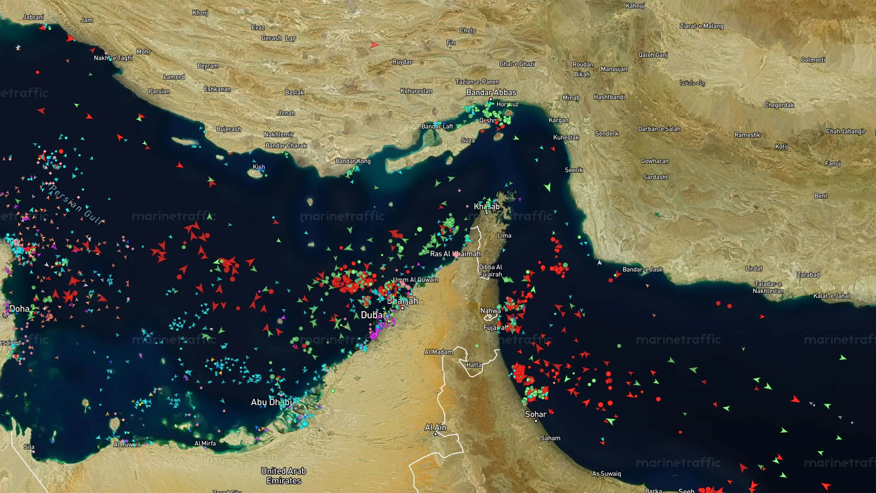
In late February 2026 Israel and the United States launched an attack on Iran. Shipping through the Strait of Hormuz at the southern end of the Persian Gulf essentially halted first because ships couldn’t obtain insurance to traverse the Strait, and later because of mines placed by Iran and blockades imposed by both sides.
While some resources are still being exported through alternate routes, the closure has had a major impact on the flow of goods around the world.
| Key Material | Quantity | World percentage | Primary Impact | References |
|---|---|---|---|---|
| Oil & Condensate | 20.9 Mbd | 21% | Transportation & Power | EIA World Oil Transit Chokepoints (2026) [EIA2026b] |
| Natural Gas | 11.4 Bcf/day | 20% | Heating & Electricity | IEA: Oil Security & Hormuz [StraitHormuz] |
| Helium | 2.5 Bcf/yr | 35-46% | Healthcare (MRI) & Tech | Intelligas: Worldwide Helium Market 2024-2029 [Wikipedia2026; USGS2026; Garvey2024] |
| Nitrogen Fertilizer (Urea) | 15-18 Mmt | 34% | Global Agriculture | IFA: Fertilizer Supply Chains & Food Security (2026) [Mills2026] |
| Sulfur | 10 Mmt | 49% | Fertilizer & Chemicals | IFASTAT: Global Fertilizer Trade Data [Mills2026; Geldard2026] |
| Ammonia | 4 Mmt | 23% | Industrial Farming | IFASTAT: Global Ammonia Trade [Geldard2026] |
| Methanol | 17.4 Mmt | 51% | Plastics & Resins | International Trader Publications: Methanol Trade 2021-2025 [JJSUDOL2025; Geldard2026] |
| Aluminum | 6.5 Mmt | 9% | Aerospace & Construction | International Aluminium Institute (IAI): Gulf Production [Wikipedia2026; Morris2026] |
| Petroleum Coke | 5-7 Mmt | 15% | EV Battery Anodes & Steel | Argus Media: Global Petroleum Coke Supply (2026) [ARGUS2026; IEA2026] |
Table: Material Impacts of the Hormuz Closure.
Two very different economic frameworks may be useful towards understand the potential economic outcome of the closure. The neoclassical view holds that production, consumption and pricing of goods and services is driven by supply and demand. Biophysical Economics (or Thermoeconomics) [Hall2018; Smil2017; Ahmed2025] says that society uses energy and biological and physical resources to generate goods and services, resulting in various forms of waste (including heat) and environmental impacts.
Mainstream economists often reject or ignore biophysical economic theory because it fundamentally contradicts the core, neoclassical assumptions of endless economic growth, market-driven substitution of resources, and the exclusion of biophysical constraints from economic models. Biophysical economics, which asserts that economic activity is a physical process governed by thermodynamics, threatens the methodological foundation and “market-centric ideology” of mainstream economics [Hoffman2012]. Herman Daly, senior economist for the World Bank and member of the Center for the Advancement of the Steady State Economy, [CASSE2024] was a strong proponent of biophysical economics.
The Neoclassical Model
The neoclassical approach to oil markets is based on a result published by Harold Hotelling in 1931. Hotelling asked: how should a rational owner of an exhaustible resource decide when to extract it? The answer, in its simplest form, is that the net price of the resource of price minus marginal extraction cost must rise at the rate of interest. If it rose faster, owners would delay extraction to capture higher future rents. If it rose slower, they would accelerate extraction to invest the proceeds. In an efficient exploitation of a non-renewable resource, the percentage change in net price per unit of time should equal the discount rate in order to maximize the present value of the resource capital over the extraction period. Hotelling’s Rule [Hotelling1931] is,
where is the price, is the marginal cost and is the interest rate. The dots indicate a rate of change so is the rate of change of the net price. Hotelling’s Rule says that markets will optimally ration the flow of oil using a price mechanism alone.
The modern neoclassical oil shock literature extends this framework into general equilibrium. James Hamilton’s 1983 paper Oil and the Macroeconomy since World War II [Hamilton1983] found that oil price shocks have been responsible for long swings in the real price of oil, notably in 1973/74, 1979/80 and 2003–2008, [Bornstein2017] and initiated research into Dynamic Stochastic General Equilibrium (DSGE) models incorporating energy as a factor of production. The key insight from Kilian’s 2009 article [Kilian2009b] is that shocks to the flow demand for oil associated with the global business cycle have been responsible for long swings in the real price of oil [Kilian2009], while speculative demand shocks can cause large immediate price effects that resolve more quickly.
The Hotelling framework has evolved to feature the geological and engineering constraints that limit the responsiveness of oil supply to price. Applied to the Hormuz closure, the neoclassical model expects the following response:
- Price signal. Closure reduces supply. Prices spike to 140/bbl within weeks.
- Supply response. High prices incentivize non-Gulf producers to accelerate output. US shale, North Sea, and Canadian operators expand drilling within 6–18 months.
- Demand destruction. At elevated prices, consumers substitute, reduce consumption, or defer purchases. GDP contracts modestly.
- Equilibrium restored. Within 6–12 months, supply and demand re-balance at a somewhat higher price level. The disruption is recorded as a transient GDP shock, roughly comparable to 1973.
The key assumption relies on the fungibility of oil. If Gulf heavy/sour crude is unavailable, light/sweet crude is an adequate substitute. If Gulf volumes are unavailable, other producers will expand to fill the gap. Price is the information mechanism that makes this work, and markets are presumed to process that information efficiently.
Oil’s contribution to global GDP is 2–3%, which lends quantitative support to the “manageable disruption” conclusion: take away something worth 2–3% of the economy and the economy contracts by something in that range, then recovers as substitutes arrive. This is the neoclassical view, while the biophysical approach argues that energy has a multiplier effect that carries through the entire economy. Food production, similarly, is modeled as a small fraction of GDP. The loss of fertilizer precursors shows up as a modest price increase in agricultural commodities, absorbed by markets within one or two growing seasons.
The neoclassical framework has been used to characterize the 1973, 1979, 1990, and 2008 oil shocks after the fact, using structural vector autoregression (VAR) models [Milvus2026] that decompose price movements into supply and demand components [Kilian2009b; Hamilton1983]. This is not the same as demonstrating that markets cleared efficiently through the price mechanism as theory predicts. Within the neoclassical literature itself, whether oil supply shocks caused the 1970s stagflation or whether monetary policy was the primary driver remains contested [Barsky2004].
The biophysical model, for its part, has not been formally tested against short-duration supply disruptions; its empirical support comes from long-run correlations between cumulative GDP and energy consumption across decades [Garrett2012; Garrett2020]. The empirical literature on whether energy Granger-causes “Granger causality” is not causality in the ordinary sense. It is a statistical test for predictive precedence: does knowing the past values of variable improve your ability to forecast variable , beyond what you could forecast from ‘s own past values alone? Formally, Granger-causes if That is, adding lagged values of to the forecast reduces the forecast error for . If it does, is said to “Granger-cause” . Granger himself was careful to note this is a test of temporal precedence and incremental predictive power, not a test of physical or logical causation. Two variables can be driven by a common third cause, in which case the one that responds faster will appear to Granger-cause the other without any direct causal link between them. GDP or vice versa has produced genuinely inconclusive results for over 35 years [Stern1993; Ozturk2010]. Both frameworks have evidentiary support and empirical limitations. The difference relevant to the Hormuz closure is not which model fits historical data better, but which captures the physical mechanisms that make this disruption structurally different from those historical episodes.
Applied to the energy-GDP question, the test asks: does knowing last year’s energy consumption help predict this year’s GDP beyond what GDP’s own history would predict? If yes — energy Granger-causes GDP — this is consistent with the biophysical view that energy throughput drives economic output. If GDP Granger-causes energy instead, that is consistent with the neoclassical view that economic demand pulls energy supply.
The complication, which is why the literature has been inconclusive for 35 years, is that the result depends on:
- How energy is measured — gross energy vs. quality-adjusted final energy vs. useful work
- What other variables are included — capital stock, employment, energy prices
- Which country and time period — the result for the US 1947–1990 differs from China 1960–2007 or OECD 1995–2007
- The lag structure — energy investments in extraction and refining precede production by months to years
The Biophysical Model
The biophysical method approaches energy and economics from first principles of thermodynamics rather than from optimization theory. Its origins begin with Frederick Soddy’s 1926 [Soddy1933] critique of monetary economics, and found later in Howard Odum’s work on energy and ecosystems, and Charles Hall and Kent Klitgaard’s synthesis in Energy and the Wealth of Nations (2012). The core claim is that GDP does not drive energy consumption, but energy drives GDP. The direction of causation is reversed from the view of the neoclassical model.
The most rigorous modern formulation of this relationship comes from atmospheric physicist Tim Garrett. Starting from thermodynamic first principles, Garrett treats civilization as an open dissipative system analogous to a growing organism in that it must continuously consume energy not just to grow, but to maintain its current size against entropy. The key finding, validated across 38 years of global data, is a near-constant ratio between current primary energy consumption and the historical time integral of inflation-adjusted global economic production,
where is energy per unit wealth and is the inflation-adjusted economic production. Using 38 years of available statistics between 1980 and 2017, the ratio remained nearly unchanged at GW per trillion 2010 US dollars [Garrett2020]. In the earlier 2012 formulation using 1990 dollars, the constant’s value was milliwatts per 1990 US dollar, and it is this link that allows treatment of seemingly complex economic systems as simple physical systems.
The implication is that economic wealth is not a static quantity that simply exists, but it requires continual energy consumption for its sustenance. Like a living organism, energy is required not just to grow civilization but also to maintain its current size. Cut the energy supply and you do not merely slow growth; the accumulated capital of civilization itself begins to decline.
In Garrett’s framework, the GDP growth equation becomes:
where is cumulative global wealth (the time integral of GDP) and is the rate of return, itself a function of energy availability. The rate of return can be expressed as , where is a coefficient of nominal production related to energy throughput, and is a correction driven by environmental degradation. [Garrett2014] The thermodynamic coupling means that when oil supply is cut, falls, not through a price signal that can be arbitraged away, but through a physical reduction in the energy available to sustain and grow civilization’s material substrate.
Hall and Klitgaard draw a practical policy implication from this framework. Oil is not a commodity input that can be simply substituted when prices rise. It is the master resource, the concentrated energy carrier that makes all other economic activity possible at its current scale. The Energy Return on Investment (EROI) of oil has been declining for decades as easy reservoirs are depleted and the Hormuz closure compounds this structural decline with an acute physical disruption.
Odum’s Maximum Power Principle adds a further constraint in that biological and economic systems evolve to maximize power throughput, not efficiency. This means production will push toward the limits of available supply regardless of price signals, and that a supply constraint is not equivalent to a cost increase but is a hard ceiling on what the system can physically do.
Why the Models Give Different Predictions
The two frameworks differ on four specific points that are directly relevant to the Hormuz closure:
| Neoclassical | Biophysical | |
|---|---|---|
| Oil’s role | Commodity input, ~2% of GDP | Master resource, physical prerequisite for GDP |
| Substitutability | High — price signal finds alternatives | Low — energy quality and infrastructure are specific |
| Recovery mechanism | Market equilibration via price | Physical supply must actually recover |
| Irreversibility | Temporary shocks, mean-reverting | Some damage accumulates and does not reverse |
Table: Neoclassical vs. Biophysical Models
We use a system dynamics biophysical model derived from Garrett’s thermodynamic coupling, geologically-inferred reserve estimates, and empirical decline rates from IEA field data. [Peach2025] The neoclassical model is not wrong about the price signal, but we argue that what it misses is that the price signal cannot substitute for physical barrels of the right grade, cannot reverse reservoir damage, and cannot accelerate nitrogen fertilizer production when the precursor gas supply has been cut.
The next three sections address the three physical mechanisms that sit outside the neoclassical frame.
Mechanism 1 - Crude Quality Mismatch
The first mechanism the neoclassical model misses is that oil is not fungible. The assumption that Gulf crude can be replaced barrel-for-barrel by shale or North Sea production is chemically and infrastructurally false, and the consequences of that falsity are large enough to change the character of the disruption entirely.
Crude oil is not a single commodity. Two critical factors determine what a refinery can do with it: API gravity (a measure of density — higher numbers mean lighter, less dense oil) and sulfur content (sour means high sulfur, sweet means low). Gulf crudes — Arab Heavy, Kuwait Export, Iranian Heavy — typically fall in the range of 28–32° API and 1.5–3.5% sulfur. These are heavy, sour crudes. US shale (Permian light), Norwegian Forties, and Algerian Saharan Blend are light and sweet: 40–45° API and under 0.5% sulfur. These are not interchangeable feedstocks. They require fundamentally different refinery configurations to process [AFPM2025].
Asian refineries which take the majority of Gulf crude were built specifically for heavy sour feedstocks. They are equipped with coking units, heavy vacuum gasoil hydrocrackers, and complex desulfurization trains. European refineries similarly built out their sour crude capacity over decades of capital-intensive investment. Switching to light sweet crude is not simply a matter of preference but requires replacing or adding major processing units at a cost of hundreds of millions of dollars per refinery and a construction timeline of three to five years per unit. The refinery reconfiguration rate in the model is calibrated at approximately 8% per year meaning that even if the capital were committed immediately, full hardware adaptation across the global refining system would take over a decade
The Effective Supply Gap
This creates a gap that the standard supply-demand accounting obscures. When the EIA or IEA reports that barrels per day of Gulf production have been displaced and barrels per day of US shale could in principle compensate, they are comparing physical volumes without accounting for the quality constraint. Much of the displaced Gulf volume simply cannot be processed in the facilities that most urgently need it.
The model captures this through a quality mismatch loss term. Let CG be Gulf export capacity, be the effective closure fraction, be the pipeline bypass fraction, and be refinery reconfiguration progress (a stock that accumulates slowly from zero):
The coefficient reflects the estimated fraction of displaced Gulf crude that simply cannot be substituted at current hardware configurations. At (pipeline bypass fraction), and (no reconfiguration yet), the loss at is approximately 1.94 Mbpd, or nearly 2 million barrels per day of supply that is physically present somewhere in the global system but cannot reach the refineries built to process it. This is separate from and additional to the volume loss from the closure itself The 0.20 coefficient is a calibrated estimate; the actual fraction depends on the specific refinery mix of affected importing countries..
In a recent bne Intellinews article, “Goldman estimates that approximately 14.5mn barrels per day of Persian Gulf crude production — equivalent to 57% of pre-war output — is currently curtailed, with the vast majority of that reduction driven by precautionary measures and stock management rather than physical damage to oil infrastructure.” [Aris2026] This estimate aligns well with our assumptions for and representing a 35% overall decline in Gulf output. Iran has been permitting a few ships through the strait, which is captured in the effective closure fraction.
The Diesel Rate-Limiter
Of all the products derived from crude oil, diesel is the most consequential for what economists would call the “real” economy which moves physical goods rather than financial claims. Every farmer, miner, long-haul freight operator, and trucking company runs on diesel. Electricity can be generated from many sources, but diesel for agricultural machinery and freight has no near-term substitute at scale.
The yield differential between crude grades is critical. Heavy sour crudes yield 30–40% middle distillates (diesel, jet fuel, heating oil) when processed in coking refineries designed for them. Light sweet crudes processed in simpler refineries yield 20–25% middle distillates [IEA2025]. The remainder shifts toward lighter products such as gasoline, naphtha and liquefied petroleum gas. Gasoline markets are already largely in balance, but the diesel shortfall will likely have the greatest impact on the world economy.
At 85% closure, the diesel shortage is not 21% (the Gulf’s share of world crude), but is closer to 20–35% of middle distillate supply depending on the configuration of refineries in the affected importing regions. Diesel trades on a separate market from crude, and when the distillate premium over crude rises significantly and holds for more than six months, it is the empirical signal that the quality mismatch mechanism is operating rather than a simple volume shortage.
Gulf crude typically yields approximately 60% middle distillates — diesel, jet fuel, and heating oil — compared with around 40% for the light/sweet shale alternatives now available. When Asian refineries substitute one for the other, they lose roughly one-third of their diesel and jet fuel output per barrel processed. Applied to the nearly 8 Mbpd of medium-sour crude that Asian refiners could no longer source in March 2026, this grade-switching penalty translates to an estimated 1.8–2.0 Mbpd shortfall in global middle distillate supply — approximately 6–7% of world diesel and jet fuel production. [HP2026; IEA2026]
We return to this point in the final section.
Mechanism 2 - The Sulfur-Nitrogen Chain
The second mechanism connects the oil disruption to systems that appear, at first glance, to be entirely separate: fertilizer production, critical mineral extraction, and the energy transition We argued previously that an energy transition is not likely even without the Persian Gulf disruption.. Sulfuric acid and ammonia are among the highest-volume substances produced by modern civilization and whose production is tightly coupled to Gulf resources.
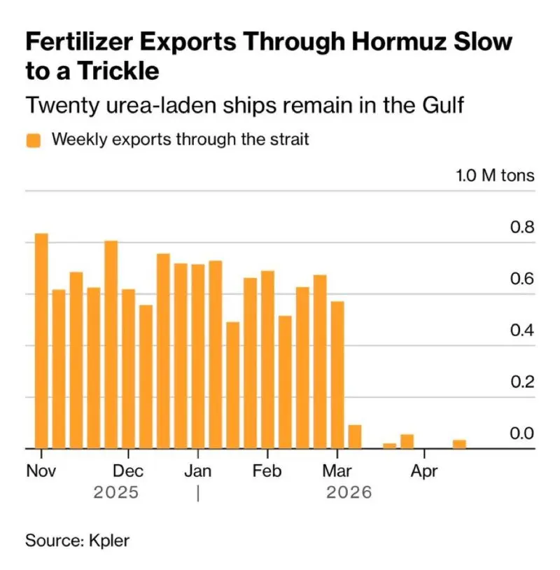
Reduction in fertilizer shipments.
Sulfur from Sour Crude
Gulf crude is sour. Removing sulfur from it before refining, called hydrodesulfurization, is not optional; it is required to meet fuel specifications and to protect downstream processing equipment. The sulfur removed in this process is recovered as elemental sulfur, which then enters global sulfur markets. The Gulf accounts for approximately 49% of internationally traded elemental sulfur [Geldard2026].
When Gulf crude stops flowing, Gulf desulfurization stops. Sulfur production falls proportionally:
At sulfur availability falls to 0.533, or a 47% reduction. The floor of 0.2 represents the irreducible minimum from non-Gulf sour crude producers (Russia, Venezuela, Canada) that continue operating The 0.55 coefficient which is the actual sulfur share from Gulf desulfurization varies with crude quality mix and is not publicly reported at the required granularity..
Sulfuric Acid and the Critical Minerals Cascade
Elemental sulfur’s primary use is not direct application, but its conversion to sulfuric acid is the single highest-volume industrial chemical in the world by tonnage. Approximately 80–90% of sulfuric acid production goes to phosphate fertilizer manufacturing and the remainder goes to hydrometallurgy, where it is indispensable [USGS2026].
Extracting copper from low-grade oxide ores by solvent extraction and electrowinning (SX-EW) requires approximately 1.5–3 metric tons of sulfuric acid per ton of copper produced. Lithium extraction from spodumene requires sulfuric acid roasting. Nickel and cobalt from laterite ores which are the dominant future source for both metals require acid leaching. Every electric vehicle, utility-scale battery, solar panel, and wind turbine requires copper; the batteries require lithium, nickel, and cobalt. There is no substitution pathway that bypasses sulfuric acid within any relevant time frame [IEA2025].
The combined effect on critical mineral supply is seen in three multiplicative constraints — sulfur/ availability, Gulf aluminum and gallium (the Gulf produces approximately 8–9% of global aluminum, and Australia, whose bauxite supply is diesel-dependent, provides feedstock for 26% of world production) [Wikipedia2026], and the indirect effects of the diesel shortage on mining operations worldwide:
where SA is sulfur availability. At representing a 40% reduction in critical minerals supply. Previously, we established that the energy transition was already physically constrained because mineral extraction rates are 100 to 10,000 times below what IPCC scenarios require. The Hormuz closure compounds a problem that was already severe.
Nitrogen and the Haber-Bosch Process
Qatar is the world’s largest exporter of liquefied natural gas (LNG), shipping approximately 77 million metric tons per year, of which 34% of global urea production depends on feedstock that transits Hormuz. [Mills2026] Natural gas is the feedstock for the Haber-Bosch process, the industrial synthesis of ammonia (NH₃) from atmospheric nitrogen:
The hydrogen comes from steam methane reforming of natural gas. Approximately 1.8 metric tons of LNG equivalent are required per ton of ammonia, and ammonia is the precursor to urea, ammonium nitrate, and all major nitrogen fertilizers. Roughly half of the nitrogen atoms in the proteins in a modern human body passed through a Haber-Bosch plant [Smil2004]. The process feeds approximately half the world’s population by enabling crop yields that would be impossible on available arable land without synthetic nitrogen.
The model captures Qatar’s LNG exposure through:
At , LNG availability falls to 0.745. The floor of 0.4 represents continued supply from US, Australian, and Russian LNG terminals on routes that do not transit Hormuz. The combined effect on food production capability, integrating nitrogen, sulfur, and diesel availability, is addressed in Mechanism 3.
Mechanism 3 - Irreversibilities
The first two mechanisms describe constraints that are severe but, in principle, reversible: open the strait and oil flows again, sulfur recovers, LNG resumes. The third mechanism describes damage that is not reversible on any policy-relevant timescale. It operates through two distinct pathways, the physical deterioration of oil reservoirs under conditions of investment neglect, and the depletion of geological oil reserves that was already in progress before the closure began.
Reservoir Neglect
Gulf oil fields are not passive storage tanks. They are complex, engineered systems that require continuous active management to maintain pressure and flow rates. Water injection sustains reservoir pressure as oil is extracted. Gas reinjection controls associated gas and maintains the energy to push oil toward wellbores. Sand control, corrosion inhibition, and scale prevention protect downhole equipment and casing integrity. When production stops, or more precisely when the revenue that funds these operations stops, the maintenance stops with it.
The consequences compound over time in a way that is qualitatively different from a temporary shutdown. In the first months, wellbore conditions deteriorate but the reservoir itself is largely intact. After one to two years without water injection, pressure gradients flatten and some zones begin to water-flood irreversibly. Water invades pore spaces previously occupied by oil and cannot be easily displaced back. After three to five years, gas cap expansion into the oil column causes permanent changes in fluid contacts. Formation damage, scale buildup in perforations, and casing corrosion accumulate. When the closure ends and investment resumes, the reservoir that operators return to is not the one they left.
The model represents this through an accelerated decline rate during closure:
where is the maintained decline rate (investment in place), is the neglect acceleration coefficient, and is the investment fraction which under closure falls to near zero because there is no export revenue to fund it. The neglect stock accumulates at the closure rate:
After approximately 3.5 years at 85% closure, crosses the threshold at which permanent physical damage begins through gas cap invasion, formation flooding, and irreversible permeability reduction. The Permanent Loss Fraction (PLF) then begins accumulating:
After a five-year closure the or a 4.5% permanent reduction in Gulf production capacity that persists indefinitely after reopening. At a ten-year closure, permanent loss reaches the 20–25% range. The model reflects the engineering literature on reservoir damage from production cessation in carbonate and clastic Clastic rocks are sedimentary rocks formed from broken pieces (clasts) of pre-existing rocks and minerals, weathered, transported, and deposited by water, ice, or wind. Classified by size—gravel, sand, silt, or clay—they include sandstone, shale, and conglomerate, typically cemented together in layers. These rocks are crucial for locating water and oil. reservoirs [Garrett2012] The specific coefficients 3.0 yr threshold and 7.0 yr full-damage period; these are calibrated estimates based on general reservoir engineering literature rather than field-specific data for Gulf reservoirs, which is not publicly available at the required resolution..
The production figure shows that by year 10, the five-year closure scenario produces approximately 2–3 Mbpd less than the open scenario even though the strait has been open for five years by that point. That gap caused by reservoir neglect is equivalent to losing Libya’s entire pre-crisis production permanently.
Peak Oil Depletion
The closure is not happening during a stable period for global oil production. The world’s conventional oil resource base has been declining in quality and quantity for decades, and the closure acts as an accelerant on a trajectory that was already unfavorable. Reservoir damage will only compound the inevitable geological reduction in output.
The model uses a geologically-inferred method to estimate the Ultimately Recoverable Resource (URR) for conventional crude. The cumulative discoveries series fitted from historical field data plateaued around 2,210 Gb in the mid-2000s. Cumulative production has crossed 1,532 Gb. Remaining reserves are approximately 678 Gb, broadly consistent with Rystad Energy’s 2P estimate of 738 Gb [Rystad2024]. At current production rates of approximately 35 Gb/yr, this represents roughly 19 years of supply at present consumption. As we showed earlier, new discovery replacement was only 9.4% of production in 2024.
This structural decline drives a depletion-linked price floor in the model:
where Gb is initial remaining URR and is the current remaining resource. As declines, the floor rises. By year 10 of any scenario, the structural price floor reaches approximately $112/bbl which is entirely independent of the Hormuz situation. The oil price cannot return to $80, not because of the crisis, but because the cheapest oil has already been produced.
The non-Gulf decline rate reflects the same depletion dynamic. The U.S. shale response to high prices is constrained by the geological reality that US tight oil production peaked in December 2025 and is projected to decline through 2026 regardless of price signals [Berman2026]. The model’s shale contribution represents the best-case offset against this baseline decline, not net new supply.
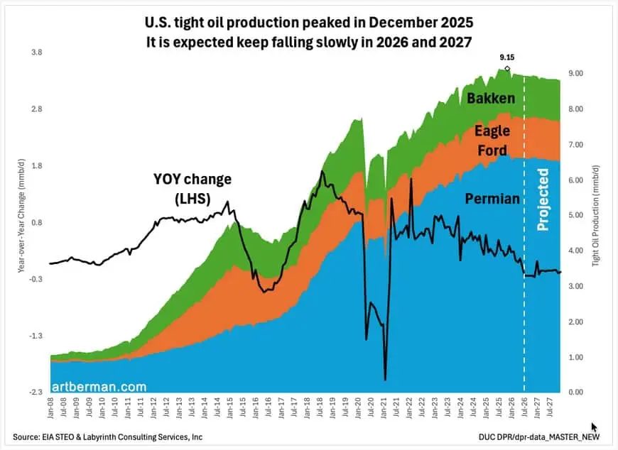
U.S. tight oil production peaked in December 2025.
The model incorporates a three-stage delay representing exploration, permitting, and drilling, and further reduces U.S. shale output which is declining at approximately 0.3 Mbpd/year from geological depletion, meaning high oil prices can partially offset but not reverse the underlying decline. This ceiling reflects physical constraints on rig availability, pipeline takeaway capacity, and the geological reality that the Permian and other tight oil plays are already producing at or near their sustainable maximum rates. [EIA2026] The heavy sour crude supply gap of 12 Mbpd from the Gulf cannot simply be replaced by other sources.
The Compounding of All Three Mechanisms
The three mechanisms do not operate independently. They interact through shared physical infrastructure and shared time. Quality mismatch means that physical barrels sitting in storage or being produced in the United States cannot reach the refineries in South Korea, Japan, Germany, and China that need them. The sulfur shortage constrains food and mineral production simultaneously. Reservoir neglect accumulates continuously while the other disruptions are playing out, and the depletion floor ensures that even full reopening cannot restore the pre-crisis price environment.
The standard linear analysis evaluates each mechanism in isolation and sums the effects. The system dynamics approach models them as a coupled system with feedbacks. GDP contraction from high oil prices reduces the investment available to accelerate the shale response, which may not be possible in any case if U.S. shale production has peaked due to geological constraints. Food insecurity from nitrogen and sulfur constraints puts additional pressure on governments already managing the economic disruption from high energy costs. These interactions are not additive but are instead multiplicative. The next section describes how the model is constructed to capture this compounding.
The Model
Understanding why the three mechanisms described above compound rather than simply add requires a modeling approach that includes time delays and irreversibilities. The method, called System Dynamics (SD), was originally developed by Jay Forrester at MIT in the 1950s and extended by John Sterman in Business Dynamics, System Thinking and Modeling for a Complex World. [Sterman2000] SD represents the world as accumulations (stocks) connected by rates of change (flows), with algebraic relationships (auxiliaries) and feedback loops linking them. The method excels where cause and effect are separated in time, where damage accumulates irreversibly, and where feedback loops create nonlinear dynamics that cannot be inferred from historical correlations alone. Neoclassical models fail to fully account for these critical feedbacks.
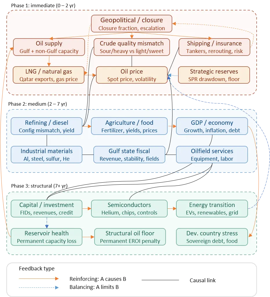
Hormuz closure system dynamics model (partial).
Architecture
The model is implemented in Julia [Bezanson2017] using ModelingToolkit.jl [Rackauckas2026] for symbolic equation specification and OrdinaryDiffEq.jl [Rackauckas2017] for numerical integration. It contains 39 variables in total: 8 main stocks, 3 delay stocks implementing a third-order material delay for the shale production ramp, and 28 auxiliaries and flows organized into five dependency tiers.
The 8 main stocks and their initial conditions are:
| Stock | Initial value | Units | Represents |
|---|---|---|---|
| Gulf_Capacity | 17.5 | Mbpd | Gulf oil production capacity |
| NonGulf_Capacity | 82.5 | Mbpd | Rest-of-world production capacity |
| SPR_Volume | 1,400 | Mb | Combined OECD strategic petroleum reserves |
| Oil_Price | 80 | USD/bbl | Global benchmark crude price |
| GDP_Index | 1.0 | dimensionless | World GDP relative to pre-closure baseline |
| Reservoir_Neglect | 0.0 | years | Accumulated Gulf reservoir damage |
| Refinery_Reconfig | 0.0 | fraction | Progress toward heavy-to-light crude adaptation |
| URR_Remaining | 678 | Gb | Geologically recoverable conventional reserves |
Table: Model stocks and initial conditions. Mbpd = millions of barrels per day; Mb = millions of barrels; Gb = gigabarrels.
The model is driven by two exogenous scenario parameters: Strait_Closure_Fraction (the fraction of normal Hormuz throughput that is blocked, 0.85 for the baseline) and Closure_Duration (how long the closure persists, in years). All other dynamics are endogenous.
The Closure Signal
The closure is not modeled as a step function. The strait closes to its specified fraction immediately at , remains at that level for Closure_Duration years, and then reopens exponentially with a time constant Reopening_Speed of 0.25 years — representing the practical reality that minesweeping, insurance restoration, and traffic resumption take months rather than days:
where is the closure duration, yr is the reopening time constant, and is the closure fraction. The effective closure function begins at 0.85, holds there, and then decays exponentially after reopening reaching approximately 0.04 after two reopening time constants (6 months).
Gulf exports during closure are limited to what can flow through overland pipelines to bypass the strait:
where is Gulf capacity and is the pipeline bypass fraction representing the Iraq-Turkey pipeline, the Saudi East-West pipeline, and the UAE’s Fujairah export terminal The Fujairah terminal on the UAE’s east coast was built specifically to bypass Hormuz. It has a design capacity of approximately 1.5 million barrels per day but has faced infrastructure and permitting constraints that limit practical throughput below this figure. which together can carry approximately 35% of normal Gulf export volume.
Supply, Price, and SPR Dynamics
Effective supply reaching consumers is Gulf exports plus non-Gulf production plus strategic reserve releases, less the quality mismatch penalty:
The equilibrium price toward which the market adjusts is a cubic function of the demand-supply ratio capturing the nonlinear price response observed in historical shortages where the last few percent of supply shortfall drive disproportionate price increases: The cubic demand-supply ratio is a common simplification in system dynamics oil models. It produces the observed nonlinearity where small shortfalls cause large price responses — consistent with the 1973 experience where a ~5% supply reduction caused a ~400% price increase.
The actual price adjusts toward the greater of and the structural depletion floor, with a one-month price adjustment time ( yr):
A speculation premium adds dollars per barrel at closure onset, decaying with a 1.5-year time constant as financial markets price in the longer-term reality.
Strategic petroleum reserves are released only when the strait is meaningfully closed () and the SPR has not fallen below its 100 Mb operational floor. Release rate is 30% of the raw supply gap, capped at 2 Mbpd:
At the initial supply gap of approximately 12 Mbpd this exhausts the 1,400 Mb combined OECD reserve in roughly 20 months, slightly under 2 years. The IEA coordinates member countries’ SPR releases. The US Strategic Petroleum Reserve alone held approximately 365 million barrels in early 2026, reduced from its peak of 727 million barrels in 2009. The combined OECD figure of 1,400 million barrels in the model reflects the full IEA member stock. The drop visible at approximately year 2 in the production scenarios is the moment SPR release ceases and the buffer disappears.
The GDP-Energy Coupling
The GDP equation follows Garrett’s thermodynamic framework rather than a price-shock response. GDP is not merely affected by oil prices; it tracks physical oil throughput with a delay, because GDP is the economic expression of energy throughput and not the other way around:
where is the GDP index (1.0 at baseline), year is the adjustment lag, /yr is the normal growth rate, and is the production ratio relative to the 100 Mbpd baseline. The first term pulls GDP toward the production ratio. If production falls to 0.88 of baseline, GDP is attracted toward 0.88 with a one-year lag. The second term provides normal growth scaled by how much physical throughput is available to support it. When , the equation reduces to simple exponential growth at 2.5%/year. When falls below 100, both terms work to push GDP downward.
This formulation implies that GDP recovery after the strait reopens is not instantaneous, but is limited by the rate at which physical supply actually recovers, which is in turn limited by reservoir damage, non-Gulf decline, and the speed of the shale ramp.
Reservoir Neglect and Permanent Loss
Gulf capacity declines at a baseline rate of 4%/year when fully maintained. Under closure conditions, investment collapses because there is no export revenue to fund it. The investment fraction is,
Even if oil prices are high, zero revenue from zero exports means zero investment, which is reflected in the term. The resulting decline rate during closure becomes,
where /year and /year. At full closure, and Gulf capacity declines at 10%/year rather than 4%/year.
Reservoir neglect accumulates at the effective closure rate and triggers permanent physical damage after 3 years:
where is the Reservoir_Neglect stock in years. At the 3-year threshold, gas cap invasion and formation flooding begin to permanently reduce the oil column available for recovery. The ceiling of 25% at represents the practical maximum reservoir damage consistent with eventual (if severely impaired) recovery.
Non-Gulf Production and the Shale Delay
Non-Gulf capacity declines continuously as geological depletion erodes the resource base. As URR_Remaining falls, the Depletion_Factor falls with it, which accelerates the background decline rate of non-Gulf producers,
generating a self-reinforcing dynamic in which producing more oil today makes tomorrow’s production harder to sustain. New shale production partially offsets this decline, but only after a 9-month delay representing the sequential bottlenecks of capital commitment, rig mobilization, and well completion. is the shale production signal delayed by year, implemented in the model as a third-order material delay with three cascaded stages of 0.25 yr each.
The shale production ramp enters through a third-order material delay representing the sequential constraints of price signal recognition, permitting and rig mobilization, and actual production coming online. Each delay stage has a time constant of 0.25 years, for a total modal delay of 0.75 years (~9 months). The ceiling on shale response is -0.3 Mbpd above the pre-closure baseline, reflecting rig availability and takeaway constraints in the Permian Basin.
Calibration
The model is calibrated against 17 simultaneous assertions evaluated at with . The key checks are:
| Variable | Expected | Units | Source |
|---|---|---|---|
| Gulf_Export_Rate | ≈ 6.1 | Mbpd | Pipeline bypass capacity [EIA2026b] |
| Effective_Supply | 85–92 | Mbpd | IEA disruption scenarios [StraitHormuz] |
| Equilibrium_Price | 100–130 | USD/bbl | Historical shock comparisons [Hamilton1983] |
| Sulfur_Availability | ≈ 0.53 | fraction | Gulf sulfur share [Geldard2026] |
| Critical_Minerals_Constraint | ≈ 0.60 | fraction | Mineral supply chain analysis [USGS2026] |
| GDP_Index at | 0.88–1.05 | dimensionless | Garrett coupling; 1973 historical GDP response |
Table: Key calibration assertions at , . All 17 assertions pass within stated bounds.
All 17 assertions pass simultaneously in a single model run. The GDP check uses the baseline scenario (4-month closure) and the range (0.88, 1.05) reflects the Garrett coupling: at , Effective_Supply is approximately 94 Mbpd due to peak oil depletion, pulling GDP_Index toward 0.94 which is below the pre-closure baseline of 1.0 even without any ongoing closure.
Limitations
The model deliberately excludes several mechanisms that would make the results more severe. It does not model financial system seizure such as credit market collapse, sovereign default cascades, and bank runs that would occur if oil prices exceed approximately $150/bbl and remain there for more than 6–12 months. It does not model political instability, rationing regimes, or state failure, all of which the societal collapse literature [Jehn2025] identifies as significant amplifiers of resource disruption.
It also does not include ecological feedbacks such as ocean fishery collapse from diesel-powered fishing fleets, topsoil loss from reduced fertilizer application, or water table depletion from diesel-powered irrigation pumps that would compound the food production impact on decadal timescales.
Each of these omissions makes the model’s results optimistic relative to reality. The scenarios shown in the next section represent a lower bound on the disruption, not a central estimate. The value of the model is not in the specific numbers since all coefficients marked [Unverified] carry substantial uncertainty, but in demonstrating that the three mechanisms identified above interact in ways that make the total impact qualitatively different from the sum of its parts.
The full model source code, calibration tests, and figure generation scripts are available on Github (see Code below). All results in this article are reproducible from the tagged release corresponding to this publication.
Results
Scenarios
Six closure scenarios span the range from geopolitical resolution to sustained conflict. All scenarios share the same closure fraction () and differ only in how long that closure persists. The open scenario provides the counterfactual of what the model predicts in the absence of any Hormuz disruption.
| Scenario | Closure duration | Reopening time constant | Analogue |
|---|---|---|---|
| Open | None | — | Counterfactual; peak oil only |
| 2 month | 0.17 yr | 0.25 yr | Rapid diplomatic resolution |
| 6 month | 0.50 yr | 0.25 yr | Negotiated ceasefire |
| 1 year | 1.0 yr | 0.25 yr | Prolonged standoff |
| 2 years | 2.0 yr | 0.25 yr | Regional war |
| 5 years | 5.0 yr | 0.25 yr | Sustained conflict / failed state |
Table: Six closure scenarios. All closed scenarios share .
Oil Production: The Physical Gap
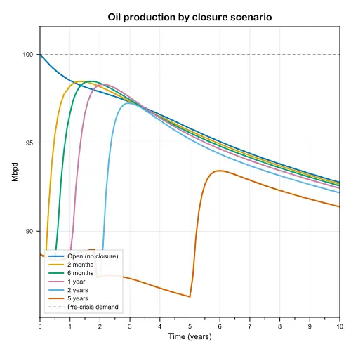
Effective oil supply reaching consumers under six closure scenarios, 2026–2036.
The most immediate physical fact of the closure is an immediate 12 Mbpd supply gap. Before the closure, the world produces approximately 100 Mbpd. At 85% closure, Gulf exports fall from 17.5 Mbpd to 6.1 Mbpd with only pipeline bypass capacity remaining. After accounting for the quality mismatch penalty, effective supply reaching compatible refineries falls to 88.7 Mbpd. The initial gap is the same at in all five scenarios no matter how long the closure lasts. The dashed line shows pre-crisis demand of 100 Mbpd. The step at approximately year 2 in all closure scenarios marks strategic petroleum reserve exhaustion.
With no closure at all, effective supply declines from 100.0 Mbpd to 92.7 Mbpd by year 10 representing a 6.8 Mbpd loss from peak oil depletion alone. Gulf capacity declines from 17.5 to 9.6 Mbpd over the same period as investment falls short of maintaining reservoir pressure in maturing fields. The Hormuz closure accelerates a supply problem that was already unavoidable.
The step visible at approximately year 2 in every closure scenario marks the exhaustion of the combined OECD Strategic Petroleum Reserve (SPR). In the 2-year scenario, the SPR drains from 1,400 Mb to its operational floor of 93.6 Mb by exactly the time the strait reopens. In the 5-year scenario, it hits that floor by year 2 and stays there for three additional years, providing no further buffer. After SPR exhaustion, the supply gap must be absorbed entirely by demand destruction which in physical terms means recession, and by whatever incremental shale production the price signal can incentivize within its possible geological ceiling of approximately -0.3 Mbpd.
The five-year closure scenario separates permanently from the others. By year 10, five years after the strait has reopened, it produces 91.9 Mbpd against the open scenario’s 92.7 Mbpd. That 1.3 Mbpd permanent gap equivalent to Kuwait’s entire pre-crisis export capacity lost indefinitely is due to reservoir neglect. The Reservoir_Neglect stock reaches 4.25 years by the time the strait reopens at well above the 3-year threshold at which permanent gas cap invasion and formation flooding begin.
Oil Price: Signal and Floor
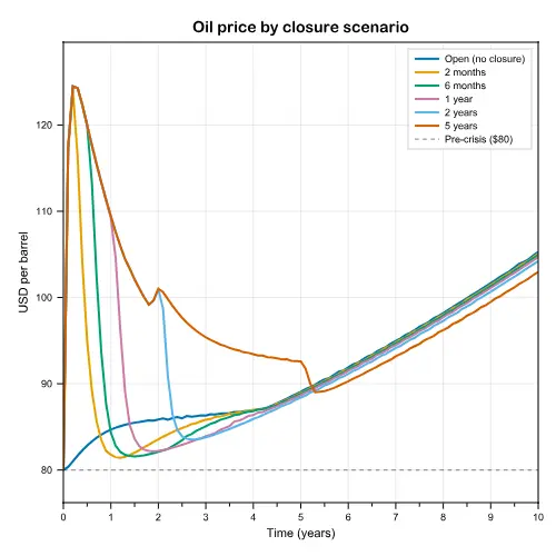
Benchmark crude oil price under six closure scenarios.
All five closure scenarios share the same price trajectory in the first six months: a spike to approximately $127/bbl by as markets absorb the supply shock and a speculation premium of $30/bbl adds to the physical shortage signal. After that, the scenarios diverge sharply based on closure duration. The dashed line marks the pre-crisis price of $80/bbl. No scenario returns to this level within the 10-year model horizon.
The short closures of 2 months and 6 months show rapid price retreat as supply recovers. The 2-month scenario returns to $81.5/bbl by year 1, tracking just above the open scenario thereafter. This is what successful neoclassical adjustment looks like in the model where the disruption is brief enough that SPR release and demand moderation bridge the gap, and the market re-equilibrates close to the pre-crisis level.
The longer closures cannot follow this path. In the 1-year scenario, price remains at $108.8/bbl at before retreating as the strait reopens. In the 2-year scenario, price at is $100.4/bbl, held down not by supply recovery but by GDP contraction reducing demand. The 5-year scenario exhibits the most counterintuitive pattern. By demand destruction is operating at scale. With the strait still closed, price has fallen to $92.7/bbl, below the 1-year and 2 year scenarios at their respective closure endpoints. The economy has contracted to a GDP_Index at 0.892 by year 5 so that demand has fallen enough to partially close the supply gap through recession rather than supply recovery.
The structural price floor is visible in all scenarios after year 3. No scenario returns to $80/bbl, but the fully open scenario reaches $105.5/bbl by year 10. This is the peak oil depletion signal as URR Remaining falls and extraction costs rise, the minimum viable oil price rises with them. A temporary geopolitical disruption can cause prices to spike and retreat but a permanent geological constraint causes prices to rise and not return. The Hormuz closure acts on top of the geological constraint, not in place of it.
The model’s price trajectories above approximately $150/bbl should be treated with caution. At sustained prices in that range, the financial system would experience credit market stress, margin calls on commodity positions, and potential sovereign default cascades in oil-importing nations, none of which the model represents. The price curves shown here are the model’s prediction of what the physical scarcity signal would be in a world where financial markets continue to function normally. The real world adds a financial seizure mechanism that would likely produce price collapses and rationing rather than smooth high-price equilibria.
Economic Output using the Garrett Model
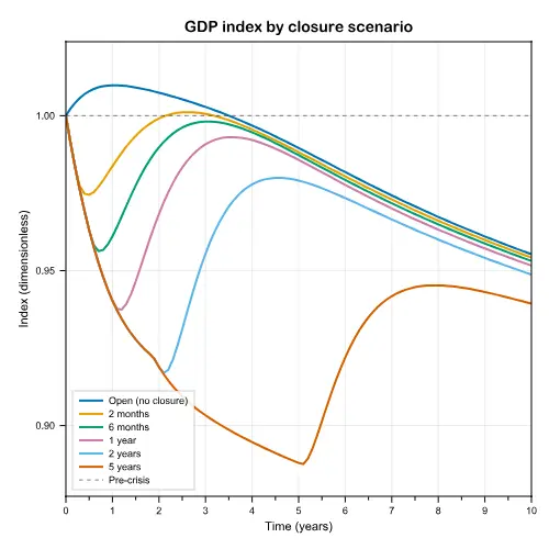
GDP Index under six closure scenarios.
The GDP results are the most important in the model, and the most important to read correctly. The open scenario with no closure and no geopolitical disruption shows GDP declining from 1.000 to 0.960 by year 10. This is due to the Garrett coupling expressing the physical reality that peak oil depletion reduces the energy throughput available to sustain civilization’s material infrastructure, independent of price or policy.
A world that successfully keeps the Strait of Hormuz open and avoids every geopolitical shock still faces a 4% GDP reduction over the next decade from resource depletion alone, according to the model. Every closure scenario is measured against this declining baseline, not against a stable one. A value of 1.0 represents the pre-closure baseline. The open scenario shows GDP declining from depletion alone, independent of any Hormuz disruption.
All five closure scenarios share the same initial GDP trajectory, GDP_Index holds at 1.000 at (the shock has not yet propagated through the 1 year Garrett lag), then falls toward the level implied by Effective_Supply. The 2-month scenario shows the mildest response with a brief dip to 0.975 at as the supply gap registers, then rapid recovery as the strait reopens and supply follows. By year 3, the 2-month scenario is indistinguishable from the open scenario.
The 5-year scenario is not recoverable in the same sense. GDP_Index reaches its trough of 0.892 at with a 10.8% decline from the pre-closure baseline, or a 6.8% decline relative to where the open scenario stands at the same point. For context, the 1973 oil shock, which disrupted approximately 5% of global oil supply for several months, caused GDP declines of 2–4% in affected economies [Hamilton1983]. The 5-year closure sustains a 12 Mbpd gap for five years, and the Garrett coupling translates this into a commensurate and lagged economic contraction.
After the strait reopens at , GDP begins recovering, but slowly, constrained by the rate at which physical supply actually returns. By year 6, GDP_Index has recovered to 0.927; by year 10, to 0.945. The gap between the 5-year closure at year 10 (0.945) and the open scenario at year 10 (0.960) is 1.5 percentage points of GDP that are simply gone and the compounded cost of five years of production suppression that cannot be retroactively made up.
The model cannot tell us what GDP contraction at this scale would mean for political stability, institutional capacity, or social cohesion. What it can say is that a 10.8% GDP decline, sustained over five years, is substantially larger than anything the post-1945 global economy has experienced outside of wartime, and that recovery to pre-crisis levels does not occur within the model’s 10-year horizon.
Food Production
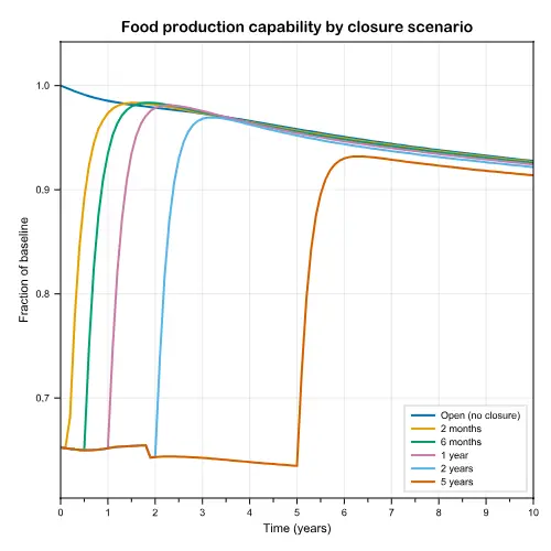
Food Production Index.
The food results reveal a structural feature that distinguishes this mechanism from the others in that the initial severity does not depend on closure duration. All five closure scenarios drop to a Food_Production_Index of 0.653 at or a 34.7% reduction in food production capability regardless of whether the strait reopens in 2 months or stays closed for 5 years. Duration determines how long the constraint persists, not how severe the initial hit is. In the figure above, Food Production Index combines LNG (nitrogen fertilizer), sulfur (phosphate fertilizer), and oil throughput (diesel for farm machinery and transport). The index measures production capability; the supply impact on food shelves arrives 6–9 months later due to harvest lag.
This uniformity has a physical explanation. Three inputs are constrained simultaneously at closure onset: LNG availability falls to 0.745 (Qatar’s export capacity severed), sulfur availability falls to 0.532 (Gulf desulfurization halted), and effective oil supply falls to 0.887 of baseline (diesel for farm machinery and transport). All three inputs are governed by the same Effective_Closure variable, which is identical across scenarios at . The Food_Production_Index is their combined product raised to exponent weights reflecting agronomic importance, nitrogen at 0.4, sulfur at 0.3, oil throughput at 0.3, and that product is the same regardless of what happens after .
The practical consequence is that the food shock cannot be avoided by a short closure. The spring 2026 planting season was underway when the closure began. Farmers made their input decisions of how much fertilizer to buy, how much fuel to budget, what to plant under conditions of supply constraint. A 2-month strait closure that ends in April still means spring crops were planted with reduced nitrogen and phosphate applications. Those crops yield what the biology allows and they cannot be retroactively fertilized after harvest. The food production impact of the current closure will not become visible in supermarket data until fall 2026 harvest figures are reported, regardless of when the strait reopens.
In the 5-year scenario, five consecutive growing seasons operate at approximately 65% of normal production capability. By year 5, Food_Production_Index has fallen marginally further to 0.638 as the ongoing production decline adds additional diesel pressure. After
reopening, food capability recovers rapidly to 0.935 by year 6, 0.919 by year 10. The failure to return to 1.0 by year 10 reflects the open scenario’s own decline. Even without the closure, food production capability falls to 0.932 by year 10 as peak oil erodes the diesel throughput underlying the final term in the food index equation.
Energy Transition Viability
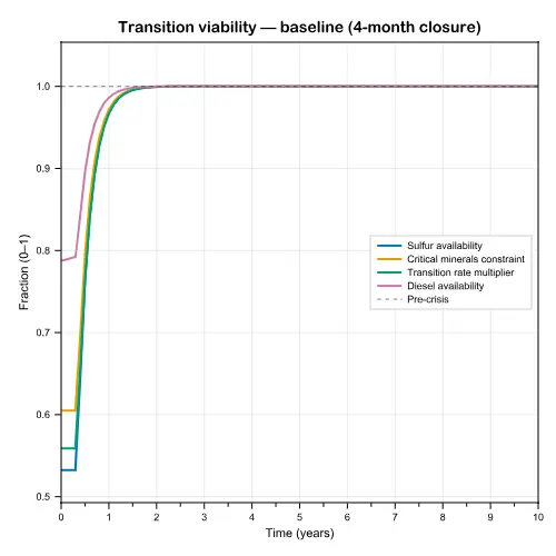
Key transition viability metrics under the baseline 4-month closure scenario.
The transition viability figure shows all metrics dropping simultaneously at . Sulfur availability drops to 0.532, the critical minerals constraint to 0.604, and the transition rate multiplier to 0.559. The physical interpretation is that the same closure that cuts oil supply to consumers also cuts the mineral supply chain inputs that the energy transition requires to build its way out of oil dependence. The dashed line at 1.0 marks pre-crisis levels. Physical supply chains recover after reopening; institutional and capital damage are not captured by this model.
At 85% closure, the world’s ability to deploy solar panels, wind turbines, and battery storage already operating far below the rate required by any credible decarbonization scenario is reduced by a further 44%. [Peach2024; Deihl2026]. As we previously established, mineral extraction rates at full pre-crisis pace were already 100 to 10,000 times below IPCC scenario requirements. The closure does not reduce a viable transition to an inadequate one, it reduces an already-inadequate rate further, while simultaneously cutting the diesel supply on which all mining and construction depends.
In any case, the concept of a transition to non-fossil energy sources has been deeply flawed. No at scale demonstration exists to support stand-alone systems permitting full reconstruction of alternative sources as components require replacement, nor have they been shown to allow expansion of energy consumption. Energy is such a valuable commodity that no substitution has ever occurred, and there is no evidence that many heavy industries such as steel and cement manufacture could continue without fossil fuel inputs. There are no viable substitutes for long-haul flights, transoceanic shipping or heavy trucking. Further, the biosphere is in rapid collapse which would likely continue with current energy consumption levels. This should not be taken as an argument in favor of continued fossil fuel consumption, but simply as a reality check on imagined energy transition scenarios.
The figure shown uses the baseline 4-month closure scenario, in which all metrics recover to pre-crisis levels within approximately 18 months as supply chains are restored. The physical recovery shown here is accurate for the supply chain inputs. What the model cannot represent is the institutional and financial damage from the disruption period. Projects canceled for lack of copper and aluminum, manufacturing capacity idled or repurposed, supply chain relationships broken, and the simple loss of 4–18 months of deployment time cannot be recovered by accelerating afterward. The physical inputs may return but the opportunity cost of the disruption does not.
Summary
The scenario data reveal a consistent pattern across all variables. The severity of the initial shock is approximately constant across all closure durations, but the consequences differ sharply based on whether the closure crosses two critical thresholds.
The first threshold is at approximately 2 years, when the strategic petroleum reserve is exhausted. Before this point, the SPR functions as a buffer that partially offsets the supply gap and moderates price and GDP impacts. After this point, the buffer is gone and further closure duration translates directly into accumulated economic damage with no offset mechanism remaining.
The second threshold is at approximately 3.5 calendar years at 85% closure, when the Reservoir_Neglect stock crosses 3 years and permanent Gulf reservoir damage begins. Only the 5-year scenario crosses this threshold, and it does so by years before the strait even reopens. This is why the 5-year scenario is qualitatively different from the others; it is the only scenario in which some of the damage is, by definition, permanent.
| Variable | Pre-crisis | yr | yr | yr | yr | |
|---|---|---|---|---|---|---|
| Effective Supply (Mbpd) | 100.0 | 88.7 | 87.8 | 86.7 | 93.9 | 91.9 |
| Oil Price (USD/bbl) | 80 | 80* | 100 | 93 | 90 | 103 |
| GDP Index | 1.000 | 1.000 | 0.921 | 0.892 | 0.927 | 0.945 |
| Food Production Index | 1.000 | 0.653 | 0.646 | 0.638 | 0.935 | 0.919 |
| Transition Rate Multiplier | 1.000 | 0.559 | 0.559 | 0.559 | 0.991 | 1.000 |
| SPR Volume (Mb) | 1,400 | 1,400 | 93 | 93 | 93 | 93 |
| Reservoir Neglect (yr) | 0.00 | 0.00 | 1.70 | 4.25 | 4.46 | 4.46 |
Table: 5-year closure scenario. Oil price at reflects the model’s 1-month price adjustment lag; the market price spike to $120/bbl occurs by . Reservoir Neglect above 3.0 years (bold) triggers permanent Gulf capacity loss.
The SPR is effectively gone by year 2 (93 Mb remaining, at its operational floor) and does not recover. Reservoir_Neglect crosses 3.0 years between and , triggering permanent damage that persists at 4.46 years even after the strait has been open for five years because the neglect stock stops accumulating at reopening but does not reverse. And GDP, Food_Production, and the Transition_Rate_Multiplier all remain below pre-crisis levels at year 10, demonstrating that the 10-year model horizon is not long enough to show full recovery for the worst-case scenario.
The data show that a 5-year closure causes lasting damage. The open question is whether the closure lasts long enough to cross these thresholds which is a geopolitical question the model is not equipped to answer.
The Canary in the Oil Well
Every model produces predictions. A model that cannot be falsified is not science; it is storytelling with equations. This section identifies one distinguishing characteristic that separates the biophysical model’s predictions from the neoclassical model’s predictions without requiring any modeling to observe.
Two Models, Two Predictions
The neoclassical model predicts a recognizable pattern: an initial price spike as markets absorb the supply shock, followed by gradual re-equilibration as the shale response materializes, demand adjusts, and strategic reserves provide a bridge. In this view, the disruption is severe but temporary. Refined product prices for diesel, jet fuel, and bunker fuel should track crude oil, staying roughly in proportion to it as they would in a normal supply disruption where the physical barrels are of the same grade as those being displaced.
The biophysical model predicts something different. If crude quality mismatch is operating, that is, if the physical barrels available cannot actually be processed by the refineries that need them most, then refined products, particularly middle distillates, should trade at an abnormally elevated premium over crude oil for an extended period. The headline crude price may moderate as demand destruction from recession pulls it down. But the diesel crack spread, the price of diesel minus the price of crude, should remain wide because the problem is not crude volume; it is the absence of the specific crude grades that yield high volumes of middle distillates.
These two predictions are distinguishable with publicly available data. Distillate crack spreads at New York Harbor averaged $1.42 per gallon in March 2026, the highest monthly level since 2022 and well above the 2021–25 five-year average of 68 cents per gallon. That is the biophysical signal already present in the data two months into the closure.
The Middle Distillate Family
The relevant signal is not diesel alone. The middle distillates — diesel, jet fuel (kerosene), and marine bunker fuel — share a common feedstock problem. All three are produced predominantly from the heavier fractions of crude that heavy/sour Gulf grades yield in abundance and that light/sweet shale grades yield in much smaller proportions. When the Gulf goes offline, all three tighten simultaneously. The crack spreads for all three should be watched together.
Diesel is the rate-limiter for the physical economy: agriculture, mining, road freight, rail. Its crack spread over Brent crude in the Amsterdam-Rotterdam-Antwerp (ARA) hub is the most globally representative middle distillate signal, reflecting European import dependence and providing the clearest read on physical tightness versus financial speculation.
Jet fuel (Jet A-1) is the rate-limiter for aviation and, by extension, for global supply chains that move high-value goods by air. Europe’s airline industry is at risk of a “systemic” jet fuel shortage in the next few weeks if the Strait of Hormuz blockade continues, with the potential of hundreds of flight cuts [Bhaimiya2026]. Middle East refineries provide Europe with around 75% of Europe’s jet fuel, and production from those facilities “is basically now almost zero,” according to IEA director Fatih Birol [Bhaimiya2026b]. The jet fuel crack spread has been the most volatile of the three: jet fuel crack spreads touched extreme levels multiple times in early 2026 — figures that only show up when buyers somewhere are genuinely short. The global price of jet fuel increased from about $99 per barrel at the end of February to as high as $209 per barrel at the beginning of April.
Marine bunker fuel is the rate-limiter for transoceanic shipping. High sulfur fuel oil (HSFO) and very low sulfur fuel oil (VLSFO) — the two dominant bunker grades — are both middle distillate products that tighten with the Gulf closure. Rising bunker costs feed directly into freight rates, which feed into the price of everything transported by sea, which is most tradeable goods.
The Six-Month Test
The distinguishing criterion is duration, not magnitude. Both models predict a spike. Only the biophysical model predicts that the spike in middle distillate crack spreads persists beyond six months.
The neoclassical logic for convergence is that non-Gulf refineries switch to available light sweet crude, increase runs, and produce sufficient middle distillates to narrow the gap within 1–2 quarters. The biophysical counter-argument, formalized in Mechanism 1, is that this substitution is hardware-constrained. Refineries cannot switch crude grades without major capital investment; the yield differential between light sweet and heavy sour crude means that even running at maximum utilization, light-crude refineries cannot produce equivalent volumes of middle distillates.
If the diesel-to-Brent crack spread at ARA, the jet fuel-to-Brent crack spread, and the VLSFO bunker-to-crude spread all remain substantially above their 5-year historical averages for more than six months, specifically, if they have not mean-reverted to within one standard deviation of their pre-crisis levels by October 2026 then the biophysical model’s account of Mechanism 1 is confirmed. In a short war scenario crack spreads collapse quickly, products correct faster than crude. During a more prolonged conflict high crack spreads persist, physical shortages, and broader inflation risks continue well into 2027.
The six-month window corresponds approximately to the time required for the fastest possible refinery switching for purchasing the necessary processing units, securing engineering contractors, and completing the first wave of hardware modifications. If crack spreads have not begun converging by that point, they will not converge until full refinery reconfiguration is complete which the model puts at approximately 8% per year, implying meaningful adaptation takes 3–5 years.
What Is Already Observable
As of late April 2026, less than two months into the closure, the following are confirmed:
The soaring cost of jet fuel is forcing European airlines to cancel tens of thousands of flights through the peak summer travel season. [Rose2026] Specifically, Lufthansa has removed 20,000 short-haul flights from its schedule through October and grounded 27 aircraft from its CityLine subsidiary. SAS has canceled 1,000 flights in April. KLM has reduced capacity by 80 flights. EasyJet has reported a headline loss of £540–560 million for the six months to March and flagged weaker forward bookings. Ryanair has warned of summer capacity cuts. Cathay Pacific has canceled approximately 2% of scheduled passenger flights from May 16 to June 30.
ACI Europe, which represents airports across the European Union, warned that if the passage through the Strait of Hormuz does not resume in any significant and stable way within the next three weeks, systemic jet fuel shortage is set to become a reality for the EU. That letter was written on April 10, 2026, but the strait has not reopened.
In August, jet fuel demand is about 40% higher than in March, so demand will increase, and if the supply stays where it is now, the challenge can be even bigger, Fatih Birol, head of the International Energy Agency (IEA), told CNBC. Peak summer aviation demand arrives in six weeks. Current jet fuel inventory trajectories, if uninterrupted, would not be sufficient to meet that demand.
Virgin Atlantic’s CEO, speaking to the Financial Times, stated the conclusion plainly: “No matter what happens in the Gulf going forward… some of this disruption to global energy prices will be here to stay.” [Campbell2026]
This is an airline CEO, someone someone who negotiates fuel supply contracts daily, telling financial markets that the neoclassical recovery narrative does not apply.
What to Watch
The three data series to monitor, all publicly available with daily updates [Petrolodex2026]:
ICE Gasoil futures minus Brent crude (the European diesel crack spread). Normal pre-crisis range: 25/bbl. Biophysical alert threshold: sustained above $35/bbl after September 2026.
Jet fuel (Jet A-1) spot price at ARA minus Brent crude (the jet crack spread). Normal pre-crisis range: 20/bbl. Alert threshold: sustained above $40/bbl after September 2026, or any regional market reporting physical allocation rather than price rationing.
VLSFO bunker price at Rotterdam minus Brent crude (the marine bunker crack spread). Normal pre-crisis range: 15/bbl. Alert threshold: sustained above $25/bbl after September 2026, combined with freight rate indices (Baltic Dry Index, Freightos Baltic Index) remaining above 150% of their 2024 baseline.
Physical rationing such as airlines being told they cannot purchase jet fuel at any price, farms being placed on diesel allocation, shipping companies unable to obtain bunker fuel at scheduled ports is a harder but more definitive signal than price alone, and should be treated as confirmation of the biophysical model regardless of where crack spreads stand at that moment [Calva2026].
The model presented in this article is falsifiable on this six-month timeline. If crack spreads have converged to historical norms by October 2026, Mechanism 1 was overstated and the neoclassical substitution story is at least partially correct. If they have not converged, if diesel and jet fuel remain structurally more expensive than crude relative to historical patterns, then the quality mismatch mechanism is operating as described, and the remaining model predictions about reservoir neglect and food supply should be treated with corresponding seriousness.
Conclusion
The Strait of Hormuz closure is being interpreted by neoclassical economists through a framework based on the 1973 and 1979 oil shocks which were demand-side rationing events responding to a supply system that was physically capable of replacing lost supply because there was spare capacity and there were alternative suppliers. The crude grades being withheld were broadly substitutable with supplies available elsewhere. The institutions that managed those crises through the release of strategic petroleum reserves, and demand reduction programs were designed for exactly that scenario.
The 2026 closure is physically different in three ways that those institutions are incapable of handling, and that the standard analytical framework does not represent.
The first difference is grade specificity. The crude that is unavailable is not being replaced by crude that refineries can process. The quality mismatch between Gulf heavy/sour grades and available light/sweet alternatives is already visible in the crack spread data. Distillate crack spreads at New York Harbor averaged $1.42 per gallon in March 2026 and are more than double the five-year historical average, while European jet fuel markets are reporting physical shortages, not just price increases.
Prices and physical shortages are different phenomena. A price increase signals scarcity and invites substitution. A physical shortage means the substitution is not happening, regardless of what price signals are sent. The airline cancellations, the ACI Europe warning letters, the IEA’s six-week jet fuel inventory statement are physical shortage signals, not price signals.
The second difference is the sulfur supply chain. The same crude that produced the world’s middle distillates also produced approximately half of the world’s traded elemental sulfur as a byproduct of desulfurization. Sulfur is the chemical precursor to sulfuric acid, which is used to make phosphate fertilizer. Sulfuric acid is also used in the hydrometallurgical processing of copper, lithium, nickel, and cobalt.
The closure has simultaneously constrained food production inputs and critical mineral supply chains. These effects are not caused by high oil prices, but are caused by the physical absence of a specific crude stream from a specific set of refineries. They cannot be resolved by releasing strategic petroleum reserves or by persuading shale producers to accelerate drilling.
The third difference is the temporal structure. The closure is not operating on a single timescale. The price spike operates on a timescale of days to weeks. The SPR buffer operates on a timescale of months and is effectively exhausted within two years at current release rates, leaving no further buffer for the remainder of any extended closure.
The agricultural lag operates on a six-to-nine-month timescale, meaning the food supply impact of spring 2026 planting constraints will not be visible until fall 2026 regardless of what happens to the strait between now and then. Reservoir neglect operates on a three-to-five year timescale before triggering permanent damage. Each of these timescales is distinct, and they overlap. The reservoir clock is running while the SPR is being depleted while the harvest is growing while refineries are running degraded feedstocks.
What Duration Determines
The model’s central finding is a threshold structure. Below approximately two years of closure, the disruption is severe but physically recoverable. The SPR bridges the worst of the supply gap, refinery operators adapt their crude slates as best they can, and the agricultural system absorbs one or two bad harvests without structural breakdown. The permanent damage in this range is limited with some reservoir neglect that accelerates Gulf decline rates, and a depletion floor that prevents oil prices from returning to pre-crisis levels.
Above approximately 3.5 years at 85% closure, the model enters qualitatively different territory. The reservoir neglect stock crosses the physical damage threshold. This is the point at which gas cap invasion, formation flooding, and infrastructure corrosion begin reducing Gulf capacity permanently. The SPR has been empty for over a year. The food shock from multiple consecutive constrained harvests has accumulated into something beyond a statistical blip.
Only the five-year scenario in this model crosses that threshold. The question of which scenario the world is actually in is a geopolitical question the model cannot answer. What the model can say is that the difference between a two-year closure and a five-year closure is not a difference of degree — it is a difference of kind.
What the Model Cannot Tell You
This model is the optimistic case. It omits financial system seizure where the credit market stress, margin calls, and potential sovereign defaults that sustained oil prices above $150/bbl would trigger in the real economy. It omits political instability and rationing regimes that would emerge as governments manage constrained energy supplies. It omits the institutional capacity decay that Kemp’s analysis of historical civilizational stress suggests follows sustained resource disruption. [Kemp2025; Ikenberry2026]
On the positive side, reduced industrial activity would relieve pressure on already-stressed ecosystems. Most commercial fisheries operate at or beyond sustainable yield; reduced fishing effort from diesel-starved fleets would allow stock recovery on a 2–5 year timescale. Reduced agricultural chemical runoff would benefit coastal dead zones. Lower freight and aviation activity would reduce marine noise pollution that disrupts cetacean navigation and feeding. These ecological rebounds would not offset the human costs of the disruption, but they are real effects the model does not capture and they cut in the opposite direction from the other omissions.
Jehn’s systematic review of the societal collapse literature identifies resource scarcity, institutional failure, and economic contraction as mutually reinforcing pathways in historical collapses [JehnOVR]. The model represents the first of these three pathways. The other two are not absent from the real world — they are absent from the model. Each missing mechanism makes the actual situation worse than the scenarios presented here.
The Falsifiable Prediction
The article makes one concrete empirical prediction that can be evaluated without any modeling. If the diesel crack spread at Amsterdam-Rotterdam-Antwerp, the jet fuel-to-Brent crack spread, and the VLSFO bunker-to-crude spread have not converged to within one standard deviation of their pre-crisis five-year averages by October 2026, then Mechanism 1, the crude quality mismatch is operating as described, and the neoclassical recovery narrative does not apply to this disruption. The crack spreads are publicly available from ICE, CME, and Platts on a daily basis.
The neoclassical model predicts that crack spreads normalize within 6–12 months as supply chains adapt and substitution occurs. The biophysical model has an equally clear prediction: crack spreads remain elevated because the substitution is hardware-constrained and cannot occur on that timescale. These predictions are mutually exclusive and empirically distinguishable.
The Larger Frame
Behind the immediate crisis lies the geological context that the cumulative discoveries data makes unavoidable. The world has consumed 1,532 Gb of conventional crude and has approximately 678 Gb remaining at geologically-inferred extraction rates. Discoveries peaked in 1964 and have replaced only ~10% of production in recent years. At current consumption rates, the remaining resource represents approximately 19 years of supply, assuming no acceleration in demand and no major disruptions to the producing regions that hold most of what remains.
The Hormuz closure does not create this constraint. The open scenario in the model still shows oil prices rising from $80 to $105/bbl by year 10 and effective supply declining from 100 to 92.7 Mbpd as geological depletion runs its course. The GDP index in the open scenario falls from 1.000 to 0.955 over the same period as the Garrett coupling transmits the production decline into economic output. The world was already on this trajectory before February 28, 2026.
What the closure has done is compress the timeline. Gulf sour crude was producing sulfur for fertilizers and industrial chemicals that most people had never heard of. Qatar LNG was feeding Haber-Bosch plants whose product ended up in the food supply of half the world’s population. Middle Eastern refineries were producing 75% of Europe’s jet fuel in a supply chain so reliable it had become invisible.
None of these dependencies appeared in the standard analysis of the Hormuz risk. The standard analysis counted barrels, while the biophysical analysis counts thermodynamic function asking: what does this flow of energy and materials actually do in the civilization that depends on it, and what happens to that function when the flow is interrupted?
The answer, visible in the crack spread data and the airline cancellation notices and the ACI Europe warning letters, is that the disruption is not primarily financial, but physical. And physical disruptions, unlike financial ones, do not resolve when confidence returns.
The only question the geopolitics will answer is how long the closure lasts. The model shows that the answer to that question will determine whether this is the worst energy crisis in modern history or the beginning of a structural reorganization of the global economy around a permanently constrained resource base.
Code for this article
The Julia code for this article is available in the GitHub repository.
Software
- Julia - The Julia Project as a whole is about bringing usable, scalable technical computing to a greater audience: allowing scientists and researchers to use computation more rapidly and effectively; letting businesses do harder and more interesting analyses more easily and cheaply.
References
- [AFPM2025] AFPM. What’s the difference between heavy and light crude oils? And why do American refineries need both?. 2025-01-24.
- [Ahmed2025] Ahmed, N. Failing States, Collapsing Systems: BioPhysical Triggers of Political Violence (SPRINGER BRIEFS IN ENERGY). 2025-10-11.
- [ARGUS2026] ARGUS. Energy Argus Petroleum Coke. 2026-04-08.
- [Aris2026] Aris, B. bne IntelliNews - Gulf oil output could recover within months of Hormuz reopening, Goldman Sachs says. 2026-04-27.
- [Barsky2004] Barsky, R. B., Kilian, L. Oil and the Macroeconomy Since the 1970s. Journal of Economic Perspectives, vol. 18, no. 4, pp. 115–134, 2004-12.
- [Berman2026] Berman, A. Requiem For An Oil Glut | Art Berman. 2026-02-10.
- [Bezanson2017] Bezanson, J., et al. Julia: A Fresh Approach to Numerical Computing. SIAM Review, vol. 59, no. 1, pp. 65–98, 2017-01.
- [Bhaimiya2026] Bhaimiya, A. Europe’s Summer Travel Season Is at Risk of a Systemic Jet Fuel Shortage. 2026-04-18.
- [Bhaimiya2026b] Bhaimiya, A. Europe’s Summer Travel Season Is at Risk of a Systemic Jet Fuel Shortage. 2026-04-18.
- [Bornstein2017] Bornstein, G., Krusell, P., Rebelo, S. Lags, Costs and Shocks: An Equilibrium Model of the Oil Industry. 2017.
- [Calva2026] CALVA, J. L. C. The Refined Products Premium: Why Diesel, Jet Fuel, Gasoline and Kerosene Have Surged Far More Than Crude Oil in the 2026 Iran War. 2026-03-24.
- [Campbell2026] Campbell, P. Virgin Atlantic boss says higher jet fuel prices are ‘here to stay’. Financial Times, 2026-04-14.
- [CASSE2024] CASSE. Herman Daly. 2024.
- [Deihl2026] Deihl, G. Sorry, No Green Revolution. 2026-04-26.
- [EIA2026] EIA. Short-Term Energy Outlook - U.S. Energy Information Administration (EIA). 2026-04-07.
- [EIA2026b] EIA. International - U.S. Energy Information Administration (EIA). 2026-03-03.
- [Garrett2012] Garrett, T. J. No way out? The double-bind in seeking global prosperity alongside mitigated climate change. Earth System Dynamics, vol. 3, no. 1, pp. 1–17, 2012-01-05.
- [Garrett2020] Garrett, T. J., Grasselli, M., Keen, S. Past world economic production constrains current energy demands: Persistent scaling with implications for economic growth and climate change mitigation. PLOS ONE, vol. 15, no. 8, pp. e0237672, 2020-08-27.
- [Garrett2014] Garrett, T. J. Long-run evolution of the global economy: 1. Physical basis. Earth’s Future, vol. 2, no. 3, pp. 127–151, 2014.
- [Garvey2024] Garvey, M. D. The 2024 worldwide helium market. 2024.
- [Geldard2026] Geldard. Beyond oil: 9 commodities impacted by the Strait of Hormuz crisis. 2026-04-01.
- [GlobalRecoverableOil] Global recoverable oil reserves hold steady at 1,536 billion barrels; insufficient to meet demand without swift electrification. 2025.
- [Hall2018] Hall, C. A., Klitgaard, K. Energy and the Wealth of Nations. 2018.
- [Hamilton1983] Hamilton, J. Oil and the Macroeconomy since World War II. Journal of Political Economy, vol. 91, pp. 228–48, 1983-02-01.
- [Hoffman2012] Hoffman, R. On the Need for New Economic Foundations: A Critique on Mainstream Macroeconomics | Cadmus Journal. 2012-10-24.
- [Hotelling1931] Hotelling, H. The Economics of Exhaustible Resources. Journal of Political Economy, vol. 39, no. 2, pp. 137–175, 1931.
- [HP2026] Hydrocarbon Processing. Asia deepens refining cuts due to Iran war, putting diesel and jet fuel supplies at risk. 2026-04-26.
- [IEA2025] IEA. World Energy Outlook 2025 – Analysis. 2025-11-12.
- [IEA2026] IEA. Oil Market Report - March 2026 – Analysis. 2026-03-12.
- [StraitHormuz] IEA. Strait of Hormuz - About. 2026-02.
- [Ikenberry2026] Ikenberry, G. J. Goliath’s Curse: The History and Future of Societal Collapse. Foreign Affairs, vol. 105, no. 2, 2026-02-17.
- [JehnOVR] Jehn, F. U. Overview Posts. 2026.
- [Jehn2025] Jehn, F. U. Systemic risk and the polycrisis. 2025-02-19.
- [JJSUDOL2025] JJSUDOL. Trends in Methanol Global Trade 2021-2025. Implications for 2026. | International Trader Publications Blog. 2026-04-17.
- [Kemp2025] Kemp, L. Goliath’s Curse: The History and Future of Societal Collapse. 2025-07-31.
- [Kilian2009] Kilian, L. Oil Price Volatility: Origins and Effects. 2009.
- [Kilian2009b] Kilian, L. Not All Oil Price Shocks Are Alike: Disentangling Demand and Supply Shocks in the Crude Oil Market. American Economic Review, vol. 99, no. 3, pp. 1053–1069, 2009-06.
- [Mills2026] Mills, R. Protect Fertilizer Supply Chains to Safeguard Global Food Security. 2026-03-16.
- [Milvus2026] Milvus. What is a vector autoregression (VAR) model?. 2026.
- [Morris2026] Morris, G. Middle East conflict harming Gulf aluminium production: IAI. 2026-04-20.
- [Ozturk2010] Ozturk, I. A literature survey on energy–growth nexus. Energy Policy, vol. 38, no. 1, pp. 340–349, 2010-01-01.
- [Peach2025] Peach, J. World Fossil Fuels Discoveries and Production. 2025-10-03.
- [Peach2024] Peach, J., Michaels, E. Burning Man. 2024-10-23.
- [Petrolodex2026] Petrolodex. 2026 Oil & Gas Market Outlook: Diesel, Jet Fuel & Gasoline Explained | Petrolodex | Crude benchmarks look calm. Product markets don’t feel calm. Here’s what’s actually driving diesel, jet fuel, and gasoline prices — and what it means for your next physical deal. | Petrolodex. 2026.
- [Rackauckas2026] Rackauckas, C. ModelingToolkit, Modelica, and Modia: The Composable Modeling Future in Julia. 2021-04-19.
- [Rackauckas2017] Rackauckas, C., Nie, Q. DifferentialEquations.jl – A Performant and Feature-Rich Ecosystem for Solving Differential Equations in Julia. Journal of Open Research Software, vol. 5, 2017-05-25.
- [Rose2026] Rose, J. Airlines in Europe slash thousands of flights as Iran war cuts jet fuel supplies. NPR, 2026-04-23.
- [Rystad2024] Rystad Energy. Global recoverable oil reserves hold steady at 1,536 billion barrels; insufficient to meet demand without swift electrification. 2024-07-26.
- [Smil2017] Smil, V. Energy and Civilization: A History. 2017.
- [Smil2004] Smil, V. Enriching the Earth: Fritz Haber, Carl Bosch, and the Transformation of World Food Production. 2004-02-27.
- [Soddy1933] Soddy, F. Wealth, Virtual Wealth and Debt: The Solution of the Economic Paradox. 1933.
- [Sterman2000] Sterman, J. Business Dynamics, System Thinking and Modeling for a Complex World. http://lst-iiep.iiep-unesco.org/cgi-bin/wwwi32.exe/[in=epidoc1.in]/?t2000=013598/(100), vol. 19, 2000-01-01.
- [Stern1993] Stern, D. I. Energy and economic growth in the USA: A multivariate approach. Energy Economics, vol. 15, no. 2, pp. 137–150, 1993-04-01.
- [USGS2026] USGS. Mineral Commodity Summaries 2026. 2026.
- [Wikipedia2026] Wikipedia. 2026 Strait of Hormuz crisis. Wikipedia, 2026-04-23.