

Extended Kelly Criterion
Handling multiple bets and payoff uncertainties
Ask NotebookLM
Introduction
Niko Tosa and a couple of his friends walked into the Ritz Club in London one night, sat down at the roulette table and broke the bank. By watching the relative positions of the ball and wheel they accurately predicted the winning pocket, and they did it without using any “cheating” methods that were used by the Eudaemons who built computers in their shoes to track the ball and wheel. Tosa won by improving the expected value of his bets in his favor. He was not only adept at predicting the outcome, but he must have studied his probability theory very carefully.
Security personnel at the Ritz reviewed the tapes of Tosa’s play, but never found evidence of any predictive software, so perhaps he was just an exceptional athlete who could sense where the ball was going. This article won’t show you how to gain an edge at roulette or any other casino game, but we’ll show you how to optimally manage your money.

Niko Tosa and his roulette strategy.
Beside predicting the outcome of each roll, Tosa likely kept careful track of how much he was betting each game. Bet too little, and he wouldn’t increase his stake at an optimum rate, but if he bet too much, he risked losing it all.
We’re not going to give you a method to pick stock market winners or encourage you to gamble, but we’ll show you how to invest wisely by managing your money. The mathematics in this article is dense, so if you’re more interested in experimenting with the outcome, go to the Github repository and download the Julia code. See the section Code for this article below for the link.
Quick Start Guide
For Mathematical Readers: Work through each section sequentially—the complexity builds deliberately.
For Experimenters: Jump to the “Experiments to Try” section, download the code, and start playing. Return to the theory when you want to understand why something works.
For Practitioners: Focus on “Discrete Case: Multiple Simultaneous Bets” and “Transaction Fees and Costs”—these have immediate practical applications.
A Review of the Kelly Criterion
In the Kelly Criterion, we showed how to optimize betting by wagering exactly the right amount of money based on the probability of winning, the expected returns, and the size of your stake at the time of the bet. Recall that if the probability of winning is the fraction of your initial capital that you bet is , and you win units per unit bet, then your wealth after bets will be
where the first term represents wins and the second losses. Letting and taking the limit as , the expected rate of return per bet is
and if we calculate the derivative with respect to , and set , we find that the optimal bet fraction is
Suppose we want to make two bets at the same time, with expected win probabilities of and , and returns and on bet fractions and . How should the bets be allocated to optimize the return?
Since and are probabilities, then , and similarly because they represent the fractions of the total current cash on hand available to bet. A further constraint is that since we can’t bet more than the total on hand.
A final constraint is that the expectation must be greater than one for each bet, so and .
Let , which is the fraction of the capital on hand after making the two bets, and , which are the amounts returned on each bet for winning outcomes. Next, let
Letting we need to find such that
Since
the value of that optimizes reduces to a function of the sum of the terms, which is cubic in , but the coefficients of the polynomial are too much for Mathematica to find a closed-form solution.
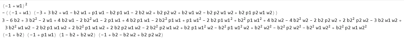
Coefficients of third degree polynomial of .
Adding in a third bet would generate a quartic polynomial, and beyond that, Abel showed that polynomials of degree five or higher have no closed form solutions (see The Sum of the Sum of Some Numbers). Still, the maximum value of exists as seen in the surface plot:
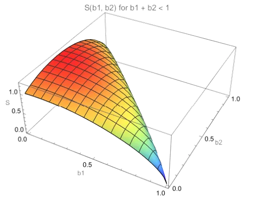
Surface plot of for .
We also need to consider cases where the payoff is a continuous probability distribution. This would be the case if you invest in the stock market and the price of the stock could, in principle, rise indefinitely, or fall to zero when the company goes bankrupt. Conversely, if you short a stock, there is no effective bottom to the losses you could incur.
For continuous probability distributions, the normal distribution is often used, but others are possible and may better represent the circumstances. We also need to consider other costs such as brokerage or exchange fees, bid-ask spreads, taxes on short-term gains, slippage, and even travel costs to casinos. These extra fees reduce the optimal betting amount and require a more conservative strategy. Many have advocated for a fractional Kelly approach where the amount bet is reduced to a percentage of the calculated optimum.
In this article, we’ll extend the Kelly Criterion in four steps:
- Discrete Case: Multiple Simultaneous Bets allows multiple bets to be placed simultaneously, but assumes winning probabilities and payoffs are known.
- Discrete Case: Uncertain Probabilities considers the situation where the probability of winning is a distribution, but the payoff is known.
- Continuous Case: Uncertain Returns investigates the case where the payoff amounts are unknown and could take on any value.
- Continuous Case: Uncertain Probabilities and Returns combines the idea that both the probability of winning and the expected payoff are distributions.
Discrete Case: Multiple Simultaneous Bets
Let’s first consider the case where the payoffs for two bets are known, and we can estimate the probabilities of winning each independently. Even though there may not be closed-form solutions for this problem, we can still find a very close numerical approximation to the optimum values for the bet fractions and . In the surface plot of , there is a maximum, and excellent numerical methods have been developed to find it. In fact, in many cases, the amount bet needs to be rounded to the nearest integer of some minimum allowable amount. For example, you couldn’t bet a fraction of a chip at a roulette table, or buy fractions of a stock.
Let’s generalize the equations to allow for an arbitrary number of simultaneous bets. Then
is the fraction of the capital remaining after the bet, and is the return amount if the bet pays. Each bet is binary - either it wins with probability or it loses with probability , and so there are possible combinations of win/loss outcomes for the bets. Let be the vector of probabilities of winning and be the vector of payoffs per unit bet. Now, if we define and the index vector to be the binary representation of an integer between and , then
where is the Hadamard, Hadamard Product: Also called the element-wise product, this operation multiplies corresponding elements of two vectors or matrices. For example, . Note that this is different from matrix multiplication or dot products. or elementwise product of vectors.
Suppose , so the index vector has values ranging from expressed in base as Using this representation, we can construct each of the terms of For example, suppose we want to generate In this case
The exponent becomes
Thus,
representing the case when the first and third bets paid, but the second lost. By constructing the function this way, we can store copies for various values of , and then optimize on the particular estimates for and at the moment we want to place a bet.
The Julia module kelly_disc.jl contains functions for optimizing the discrete case. Suppose you have two opportunities where , and If they were played independently, then the optimal bet fractions would be
When playing both bets simultaneously, the betting fractions change slightly:
============================================================
DISCRETE KELLY OPTIMIZATION RESULTS
============================================================

Problem Setup:
  Number of bets: 2
  Transaction fee: 0.00%

Bet Parameters:
  Bet 1: p=0.3000, w=4.0000, E[p·w]=1.2000
  Bet 2: p=0.2500, w=6.0000, E[p·w]=1.5000

Optimal Bet Fractions:
  b_1 = 0.064500 (6.45%)
  b_2 = 0.099154 (9.92%)

Total bet: 0.163655 (16.37%)
Cash held: 0.836345 (83.63%)

Max E[log(wealth)]: 0.028532
Converged: true  Iterations: 3  Method: lbfgs
============================================================
The long-term growth rate is per bet, so if you play similar bets, your initial stake will grow by times.
The third input parameter to DiscreteKelly is the transaction cost, which we set to zero in the example above, but should be considered in an actual betting situation. Suppose you’re playing roulette (see Roulette Physics) and you can reliably predict where the ball will fall within an octant. It might become obvious that you’re playing several numbers that are adjacent on the wheel, so to cover this, you could throw a few chips randomly onto other numbers, which would be a transaction cost. You might also include travel expenses or taxes as a transaction cost, but this would be amortized over your stay at the casino.
The DiscreteKelly function should be restricted to a handful of simultaneous bets because the number of terms in the solution equation doubles with each new bet. If you have discrete bets, then the number of terms will be since each combination of win/lose needs to be included. For example, if you have bets, then the equation will have terms.
Discrete Case: Uncertain Probabilities
Unlike the previous case, where we assumed a fixed probability of winning and a known payoff, Niko Tosa didn’t know the probability exactly, but knew only a distribution. The game is still binomial - you win with probability and lose with probability , but your knowledge of itself is uncertain. If you use a fixed value of , then you are assuming more information about the outcome than you actually have.
If you assume that the distribution is a beta distribution, Beta Distribution: A flexible probability distribution defined on the interval [0,1], controlled by two parameters ( and ) that determine its shape. When both parameters equal 1, it becomes a uniform distribution. then you can begin to estimate the parameters by collecting your win/loss results. The beta distribution is defined in the interval by
where
and is the Gamma function.

Beta distribution PDF.
Start with an initial guess for the probability , called the prior. With no knowledge of how well you will be able to predict the outcome, set , which gives equal likelihood to every pocket for an American wheel (change to 37 pockets for European). Now, begin collecting data, counting the number of wins and the total number of attempts , which will improve your estimate of the true distribution
where means “the probability given collected data”. The empirically derived probability is the mean of the distribution,
An even better way to estimate the probability distribution would be to record how far off your guess is for the winning pocket. Build a vector of distances between the estimated target pocket and the true pocket, , where represents pockets early, is exactly right, and is pockets late. Now you can use the Dirichlet distribution Dirichlet Distribution: A multivariate generalization of the Beta distribution used when modeling multiple categories that must sum to 1. Think of it as modeling probabilities for multiple outcomes simultaneously, such as the likelihood of a roulette ball landing in different groups of pockets., which is a multivariate extension of the Beta distribution, to develop a more complete model of the error pattern. As in the case with the Beta distribution, start with an estimated prior and collect counts of each offset value to estimate the posterior
Using this method provides a better estimate of the probabilities over a range of adjacent pockets. For the Dirichlet priors, the best initial estimate is for all .
We can compare how the uncertain probabilities affect the betting fraction to the prior case where we knew the probabilities of winning exactly. Let and for some small value of such as so the resulting probabilities are very uncertain. Keep the payoffs the same as previously,
s = 10.0       # weak prior, much more uncertainty about p
α1, β1 = s*p1, s*(1-p1)
α2, β2 = s*p2, s*(1-p2)
p_dists = [Beta(α1, β1), Beta(α2, β2)]
and then run the multi-Bayes example,
[0.0645002348517128, 0.09915443802025861]  total bet = 0.1636546728719714
Multi-bet Bayesian Kelly result:
  b_1 = 0.064500 (6.45%)
  b_2 = 0.099154 (9.92%)
  Cash held = 0.836345 (83.63%)
  Total bet = 0.163655 (16.37%)
  Max E[log(wealth)] = 0.028532
  Converged: true  Iterations: 8  Method: lbfgs_bayes_multi
which gives the same result as the discrete case. For a single bet with probability and log-utility, Log-Utility: Using logarithms to measure wealth changes captures the diminishing marginal value of money—doubling your wealth from to doesn’t feel as significant as doubling from to . This aligns with how humans actually perceive financial gains. the conditional expected log-wealth is
If is random with some distribution (e.g., Beta), the Bayesian expected log-wealth is
so the dependence on the distribution of vanishes except for the mean If you wanted to include a variance term, you could define the objective function as
where is a measure of your risk tolerance. Alternatively, you could run Monte Carlo simulations Monte Carlo Methods: Computational techniques that use repeated random sampling to obtain numerical results. Named after the famous casino, these methods are particularly useful when analytical solutions are difficult or impossible to find. with data collected in situ to optimize or use the method described in Distributional Robust Kelly Gambling by Qingyun Sun and Stephen Boyd.
Continuous Case: Uncertain Returns
What if we don’t know the exact return, but only its probability distribution? Instead of a fixed return , the payoff is a function where is a probability density function. In this example, the payoff reaches a maximum when , with a probability of but could also be with probability and falls away to zero for or
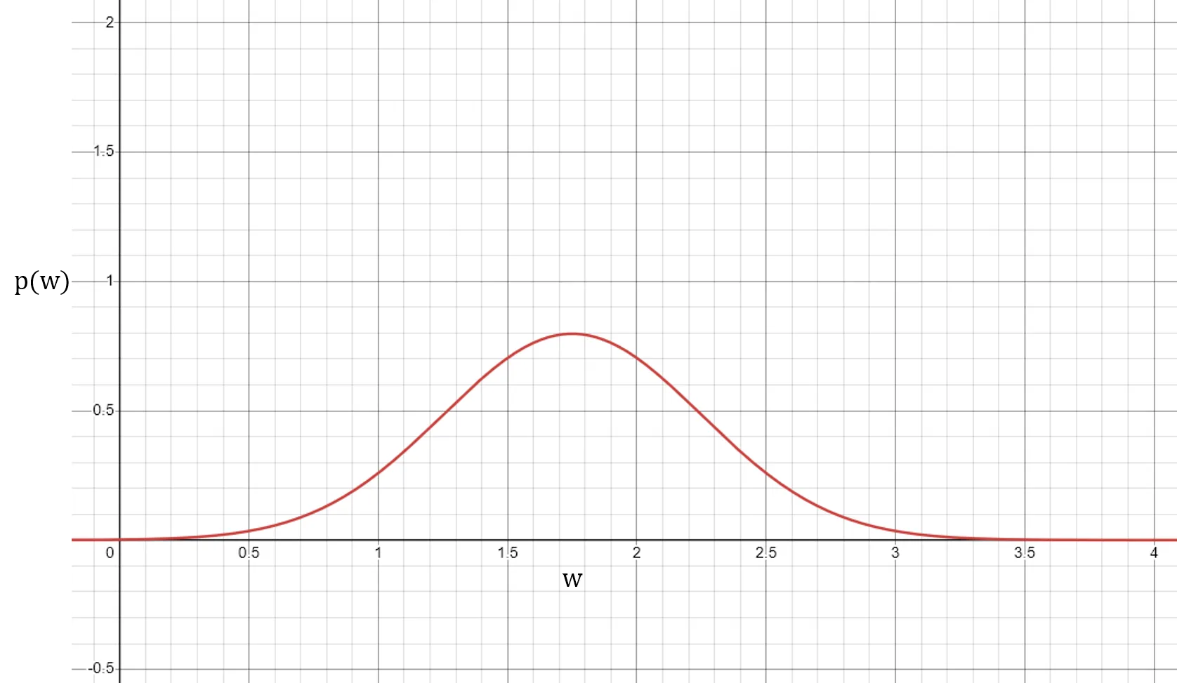
Payoff returns as a continuous distribution.
For a single bet with a continuous probability distribution, the wealth after betting is
The objective function is,
and we want to maximize This is similar to Claude Shannon’s Information Entropy discussed in The Kelly Criterion,
where is the probability of receiving message , and is the vector of messages, .
For multiple simultaneous bets with bet fractions and payoffs the wealth after one session is
The objective function for multiple bets becomes
with the constraints
Multiple Continuous Kelly
Just as in the discrete case, we can extend the continuous case to include multiple simultaneous bets. If the bets are known to be independent, as might be the case if day-trading in unrelated industries, then we could invest in multiple trades simultaneously to improve the overall probability of success.
In the example above with two bets, and we found that the optimal fractions were When the probabilities are continuous, the input parameters are dependent on the expected payoff values and the probability distribution. For the discrete case, the expected value and variance are
where is the gross return:
- with probability
- with probability .
For the first bet,
and for the second bet and
For a continuous distribution, the log-normal works well because it is bounded below by zero, so the payoff is never negative.
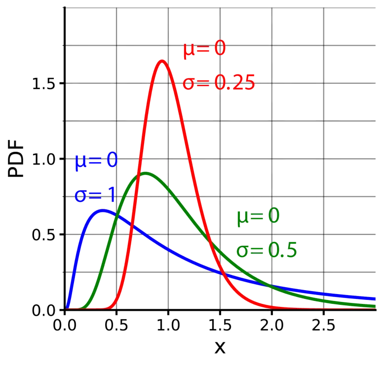
Log-normal distributions.
The expected value for a log-normal distribution is and the variance is Then
and
(See the Appendix for details on the variable .) For the first bet, and so
and for the second bet and so and
===============================================================
Number of bets: 2
Transaction fee: 0.00%
Correlation: Independent

Bet parameters:
  Bet 1: LogNormal{Float64}, μ=1.2000, σ=1.8330
  Bet 2: LogNormal{Float64}, μ=1.5000, σ=2.5981

Optimal bet fractions:
  b_1 = 0.029763 (2.98%)
  b_2 = 0.037038 (3.70%)

Total bet: 0.066801 (6.68%)
Cash held: 0.933199 (93.32%)

Max E[log(wealth)]: 0.019828
Converged: true  Iterations: 0  Method: mc_fixed
===============================================================
Notice that the bet fractions for the continuous distribution are much smaller (2.98% and 3.70%) than for the discrete case (6.45% and 9.92%). In the discrete case, the payoff is certain and only the probability of winning is uncertain, while in the continuous case, the payoff might be any value greater than zero.
The log-normal distribution has a heavy tail near zero and a much smaller tail that extends on to infinity, so the expected value is lower. The continuous Kelly reduces the bet size to reflect the reduced expected payoff.
Continuous Case: Uncertain Probabilities and Returns
In this final extension of the Kelly Criterion, we consider the case that both the probability of winning and the payoff are taken from probability distributions. The probability of winning is taken from a Beta distribution, and the payoff is a univariate distribution, and is implemented in the module kelly_general_bayes.jl, and extends the concepts developed in the previous models. This version lets you place multiple simultaneous bets allocated optimally to increase your total capital at the maximum rate, and, as in previous models, lets you include fees or betting costs.
Traditional Kelly models assume you know the probability of winning and the payoff exactly, but we can now turn both into distributions that better reflect how you would approach an investment or betting opportunity. By modeling distributions, we have a rigorous basis for adjusting the betting fractions. For example, if we use the probabilities and payoffs from the first example above,
# Fixed means and payoffs:
p1_mean, p2_mean = 0.30, 0.25
gross_w1, gross_w2 = 4.0, 6.0
and compare a strong prior, to a weak prior, in two scenarios, we see that the weak prior causes the optimal fractions to be reduced by over 15%
Scenario A (strong prior): b = [0.06565483237670092, 0.0990407051985005]  total bet = 0.16469553757520142
Scenario B (weak prior):  b = [0.044006266789879726, 0.09526125397014709]  total bet = 0.13926752076002683
Fraction reduction in total bet = 15.44%
In most cases, the reduction would likely be even greater since the expected values are high in this example, With strong conviction (tight probability prior) and near-known payoff distributions, the model recovers something very close to classic Kelly fractions, but with weak conviction (diffuse probability priors) or large payoff variance, the optimal fractions naturally shrink, reflecting risk from estimation error or payoff tail risk.
With multiple simultaneous bets, you can allocate capital not just by edge but also by uncertainty, return variability, and covariance if enabled. Here’s how to use this model:
-
Define your model beliefs
-
Choose for each bet : a prior distribution for (e.g.,
Beta(α,β)), a win and loss return distribution (e.g.,LogNormal(μ,σ)). -
Optionally, a correlation matrix if bet returns are dependent.
-
-
Instantiate the model
k = GeneralBayesianKelly(p_dists      = [ … ],
                         return_dists = [ … ],
                         loss_dists   = [ … ],
                         fee          = f,
correlation = Corr)- Optimize for stake fractions
res = optimize_gen_bayes(k; method=:lbfgs, n_samples=…, rng=…)The result res.b gives the vector of optimal bet fractions, res.cash the un-bet cash fraction, and res.objective the achieved expected log-wealth.
- Inspect and plot
Use
plot_objective_gen_bayesto explore how expected log-wealth varies with each , or compare different prior strengths and payoff variances to study their effect on allocation.
The kelly_general_bayes.jl lets you model real-world conditions much more accurately than the original single bet, fixed probability, and fixed payoff model.
You can also run Monte Carlo simulations,
include("kelly_general_bayes.jl")
using .KellyGeneralBayes
using Random

# Base model
(k, res_kelly) = run_examples_general()

# Make some alternative strategies to compare:
# e.g., half-Kelly and a "conservative" tweak
res_half = GenBayesKellyResult(0.5 .* res_kelly.b,
                               1.0 - k.fee - sum(0.5 .* res_kelly.b),
                               res_kelly.objective, true, 0, :manual_half)

res_zero = GenBayesKellyResult([0.0, 0.0], 1.0 - k.fee, 0.0, true, 0, :cash_only)

fig = compare_strategies_monte_carlo(
    k,
    ["Full Kelly" => res_kelly,
     "Half Kelly" => res_half];
    n_iters=3000,
    n_horizon=200,
    bands=((0.10,0.90),(0.25,0.75)),
    bins=40,
    rng=MersenneTwister(123)
)

display(fig)
which shows the difference between a conservative half-Kelly and the full model:
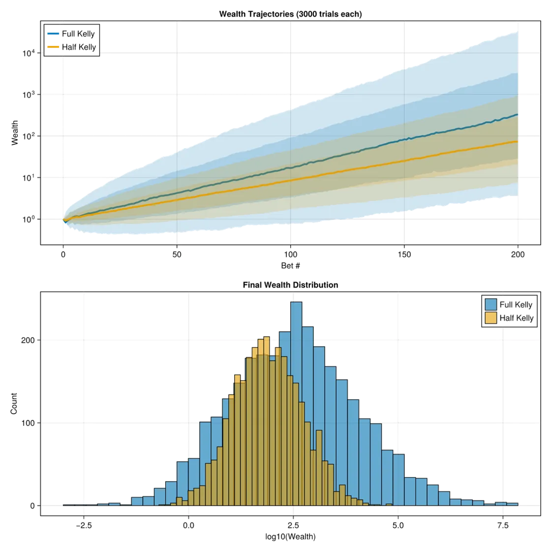
Wealth trajectories.
Transaction Fees and Costs
You need to consider various costs that might reduce your overall winnings. While playing roulette, you might spread a few “dummy” bets around the table to hide the fact that your system is consistently selecting a few winning pockets. For day trading, there are brokerage fees and taxes to consider, among others. In the code, we simply subtract the fee from available capital: to account for these losses. Some extra costs you should consider are,
- Fixed percentage fees (brokerage, exchange fees)
- Bid-ask spreads - The range between the buying and selling prices offered for a security.
- Tax on short-term gains - Tax on profits gained when a position is held for less than one year.
- Slippage - The difference between the expected price of a trade and the price at execution.
You should also consider the possibility of naturally occurring long strings of losses. Imagine playing a game involving a coin toss in which heads is a win and tails is a loss. The law of large numbers says that over many tosses, the number of heads will approximately equal the number of tails, but there will always be long runs of tails that could happen at any time. If the run is long enough, no matter how large your initial capital, you will go bust. This is known as gambler’s ruin, and we need to account for the possibility of such an occurrence.
⚠️ Common Pitfalls When Using Kelly
- Overestimating your edge - The #1 error. Kelly assumes you know probabilities accurately.
- Ignoring correlation - Betting on multiple correlated outcomes isn’t really diversification.
- Forgetting transaction costs - Even small fees dramatically reduce optimal bet sizes.
- Not rebalancing - Kelly fractions need updating as your wealth changes, preferably after each transaction.
- Using arithmetic means - Kelly requires geometric thinking about compound growth.
Possible Applications
Several investment or betting opportunities could benefit from the extended Kelly-Criterion framework:
Quantitative trading strategies / algorithmic strategies
Many algorithmic trading or systematic strategies have the following characteristics:
- You have a historical signal that suggests a trading edge (i.e., probability of success), but that probability is uncertain.
- The returns when the trade succeeds or fails are random (sometimes large winners, sometimes tail losses).
- You may run many strategies simultaneously (i.e., multiple “bets”).
Sports betting or wagering markets
In sports betting, you may estimate true win probabilities of teams or players (based on models/data) and compare them with bookmaker odds. There is inherent uncertainty in your probability estimates, and payoffs are known (or nearly known) when you win, but you can treat them as distributions if you include, e.g., parlay possibilities.
Options or derivatives trades with modelled edge
In options trading, you may have a view that an option is mispriced (so you estimate a probability of a favorable outcome), and you have an estimate of payoff distribution (the option payoff is a known structure, but the underlying volatility or tail risk is uncertain).
Summary
These extensions to the original Kelly Criterion bring you much closer to realistic betting/investing opportunities by modeling uncertain probabilities of winning and uncertain payoff amounts, optimizing over multiple simultaneous bets, and including transaction fees. The models check that your total bet fraction is never greater than one, and each bet has an expected value greater than one.
These methods only optimize the betting fractions, so you still need to accurately estimate the chances of winning and how much you expect to make on each investment. Many investments could benefit from applying the extended Kelly Criterion, but be sure to thoroughly understand each and be careful when developing the distributions used.
Where to Go From Here
The mathematics we’ve covered transforms the simple Kelly Criterion into a practical tool for real-world decision-making. But understanding the theory is just the beginning—the real value comes from experimentation and application.
Start conservative, then explore: Begin with the discrete case using small, hypothetical portfolios. Watch how the optimal fractions change as you adjust probabilities and payoffs. Notice how uncertainty in your estimates naturally reduces the recommended bet sizes—this is the model protecting you from overconfidence.
Build intuition through simulation: Run Monte Carlo simulations comparing full Kelly to half-Kelly strategies. You’ll see that while full Kelly maximizes long-term growth, it also experiences dramatic drawdowns. This visceral understanding of the volatility-growth tradeoff is something equations alone can’t teach.
Test with real data: Apply these models to historical data—stock prices, sports betting odds, or even board game probabilities. The gap between theoretical optimal betting and practical constraints will become immediately apparent. Transaction costs matter. Estimation error matters. The frequency of rebalancing matters.
Remember the limits: These models optimize how much to bet, not what to bet on. No amount of mathematical sophistication can turn a bad edge into a good one. The Kelly Criterion’s most important lesson might be knowing when not to bet at all.
The Julia code accompanying this article gives you a laboratory for exploring these ideas. Whether you’re managing an investment portfolio, analyzing strategic decisions, or just curious about optimal resource allocation, the extended Kelly framework offers a rigorous foundation for thinking about risk, uncertainty, and growth.
Start experimenting. Start small. And most importantly, start learning from what the models tell you about your own assumptions.
Experiments to Try
Ready to dig deeper? Here are hands-on experiments to build your intuition:
Beginner Experiments
-
The Overconfidence Test
- Set up two bets with p₁=0.3, w₁=4 and p₂=0.25, w₂=6
- Compare optimal fractions using strong prior (s=1000) vs weak prior (s=10)
- Question: How much do your bet sizes shrink when you’re less certain?
-
The Correlation Explorer
- Create two bets with identical expected values
- Run optimizations with correlation = 0, 0.5, and 0.9
- Question: How does correlation between bets affect diversification benefits?
-
The Transaction Cost Reality Check
- Take any optimal betting strategy
- Gradually increase the fee parameter from 0% to 5%
- Question: At what fee level does the strategy become unprofitable?
Intermediate Experiments
-
Discrete vs Continuous Comparison
- Set up the same scenario using both discrete and continuous models
- Compare the optimal fractions (you’ll see continuous gives smaller bets)
- Question: Why does uncertainty in payoff reduce bet size more than uncertainty in probability?
-
The Gambler’s Ruin Simulator
- Start with $1,000 and a favorable bet (p=0.55, w=2)
- Use full Kelly fractions for 1,000 rounds
- Run 100 simulations and plot the distribution of outcomes
- Question: How many simulations went bust despite positive expected value?
-
Half-Kelly vs Full Kelly Battle
- Run 10,000 iterations comparing both strategies
- Track: median wealth, maximum drawdown, probability of 50% loss
- Question: Is the extra volatility of full Kelly worth the higher growth rate?
Advanced Experiments
-
Multi-Asset Portfolio Optimization
- Create 5 independent betting opportunities with varying risk/reward
- Optimize simultaneously vs optimizing each independently
- Question: How much does simultaneous optimization improve expected growth?
-
Bayesian Learning Simulation
- Start with a weak prior (Beta(1,1)) for win probability
- Simulate 100 bets, updating your belief distribution after each
- Watch optimal fractions evolve as your estimates improve
- Question: How many observations until your bets stabilize?
-
Stress Testing with Fat Tails
- Replace log-normal return distribution with Student’s t-distribution (df=3)
- Compare optimal fractions to the log-normal case
- Question: How should you adjust betting when extreme outcomes are more likely?
-
The Rebalancing Frequency Study
- Set up a two-bet continuous strategy
- Compare: rebalance every bet vs every 10 bets vs never rebalance
- Question: How much growth do you sacrifice by not rebalancing?
Real-World Application Challenge
- Your Own Portfolio Analysis
- Take 3-5 investments you’re considering (or currently hold)
- Estimate probability distributions for each using historical data
- Run the general Bayesian Kelly optimization
- Compare recommended fractions to standard “equal weight” or “market cap weight”
- Question: How different are Kelly-optimal weights from conventional wisdom?
Debugging Your Intuition
- The Impossible Bet Exercise
- Try to optimize a bet with p=0.4, w=2 (expected value < 1)
- Watch the optimizer recommend b=0
- Try p=0.5, w=2.1 (barely favorable)
- Question: How close to break-even must you be before Kelly says “don’t bet”?
Documentation and Sharing
For each experiment:
- Record your hypothesis before running
- Document unexpected results
- Share interesting findings in the GitHub discussions
The best way to learn Kelly optimization isn’t through equations—it’s through breaking the models, stress-testing assumptions, and discovering edge cases. Start experimenting today.
Glossary
- Kelly Criterion: A betting strategy that maximizes the long-run geometric growth rate.
- Fractional Kelly: Betting a fraction of the full Kelly amount to reduce risk.
- Expected Log Wealth: The objective function Kelly maximizes.
- Value at Risk (VaR): The maximum loss at a given confidence level.
- Conditional VaR (CVaR): Expected loss given that loss exceeds VaR.
- Maximum Drawdown: Largest peak-to-trough decline in wealth.
- Sharpe Ratio: Risk-adjusted return metric (mean/std dev).
- Probability of Ruin: Chance of going bankrupt.
- Rebalancing: Adjusting portfolio to maintain target allocations.
- Geometric Mean: nth root of the product of n values (appropriate for compounding).
- Arithmetic Mean: Sum of values divided by count (not appropriate for Kelly).
Code for this article
The complete Julia implementation is available at Extended Kelly Criterion — Julia Implementation. The code for each section is
kelly_disc.jl- Discrete multiple bet optimizationkelly_bayes.jl- Bayesian uncertain probabilitieskelly_cont.jl- Continuous return distributionskelly_general_bayes.jl- Full general case
This repository provides a full suite of four standalone Kelly-optimization models, progressing from classical fixed-probability betting to general Bayesian optimization with uncertain probabilities and uncertain return distributions.
Each module is self-contained: optimization routines, Monte Carlo tools, plotting utilities, and examples are implemented within each .jl file—no external utility files are required.
Software
- Julia - The Julia Project as a whole is about bringing usable, scalable technical computing to a greater audience: allowing scientists and researchers to use computation more rapidly and effectively; letting businesses do harder and more interesting analyses more easily and cheaply.
- Wolfram Language - Wolfram Language is a symbolic language, deliberately designed with the breadth and unity needed to develop powerful programs quickly. By integrating high-level forms—like Image, GeoPolygon or Molecule—along with advanced superfunctions—such as ImageIdentify or ApplyReaction—Wolfram Language makes it possible to quickly express complex ideas in computational form.
References
- Andersen, R., et al.. In-game betting and the Kelly criterion. Mathematics for Application, vol. 9, no. 2, pp. 67–81.
- Beta distribution. Wikipedia.
- Bhowmick, K.. Inverse Problems in Portfolio Selection: Scenario Optimization Framework.
- Browne, S., Whitt, W.. Portfolio Choice and the Bayesian Kelly Criterion.
- Carta, A., Conversano, C.. Practical Implementation of the Kelly Criterion: Optimal Growth Rate, Number of Trades, and Rebalancing Frequency for Equity Portfolios. Frontiers in Applied Mathematics and Statistics, vol. 6.
- Carta, A., Conversano, C.. Practical Implementation of the Kelly Criterion: Optimal Growth Rate, Number of Trades, and Rebalancing Frequency for Equity Portfolios. Frontiers in Applied Mathematics and Statistics, vol. 6.
- Chellel, K.. Meet the Man Who Proved Roulette Was Beatable. Bloomberg.com.
- Dirichlet distribution. Wikipedia.
- Gordon, G., Tibshirani, R.. Karush-Kuhn-Tucker conditions.
- https://byjus.com/maths/beta-distribution/.
- Jonathan. Hey Kelly, Optimize My Portfolio.
- Karush-Kuhn-Tucker Condition - an overview | ScienceDirect Topics.
- Kelly, J. L.. A New Interpretation of Information Rate.
- Kim, S. K. (.. Kelly Criterion Extension: Advanced Gambling Strategy. Mathematics, vol. 12, no. 11.
- Kirschenmann, T.. thk3421-models/KellyPortfolio.
- MacLean, L. C., et al.. Good and bad properties of the Kelly criterion.
- MO-BOOK: Hands-On Mathematical Optimization with AMPL in Python 🐍 — Hands-On Mathematical Optimization with AMPL in Python.
- Multivariate Optimization - KKT Conditions.
- Niko Tosa Roulette Strategy vs. Traditional Approaches.
- Numerically solve Kelly criterion for multiple simultaneous bets.
- Peterson, Z.. Kelly’s Criterion in Portfolio Optimization: A Decoupled Problem.
- philh, et al.. When and why should you use the Kelly criterion?.
- Reid, A.. Kelly Criterion: The Smartest Way to Manage Risk & Maximize Profits.
- Sizing the bets in a focused portfolio.
- Sun, Q., Boyd, S.. Distributional Robust Kelly Gambling.
- The Gambler Who Beat Roulette and Made History.
- Thorp, E. O.. Chapter 9 The Kelly Criterion in Blackjack Sports Betting, and the Stock Market. Handbook of Asset and Liability Management, vol. 1, pp. 385–428.
- Thorp, E. O.. PORTFOLIO CHOICE AND THE KELLY CRITERION. World Scientific Handbook in Financial Economics Series, vol. 3, pp. 81–90.
- Understanding a Wager: To gamble or not to gamble, that….
- Wesselhöfft, N.. The Kelly Criterion: Implementation, Simulation and Backtest.
- Ziemba, D. W. T.. Understanding the Kelly Capital Growth Investment Strategy.
Image credits
- Hero image: DreamStudio.
- Niko Tosa: Roulette equations by Irene Suosalo. In BetUS, Niko Tosa Roulette Strategy vs Traditional Approaches.
- Surface plot of - screenshot from Mathematica computation
- Beta distribution: By Horas based on the work of Krishnavedala.
- Payoff returns as a continuous distribution - Desmos.
- LogNormal distribution: By Xenonoxid.
Appendix
What is ?
In the equation
the symbol is just a temporary variable used to simplify the algebra. It represents the multiplicative ratio
For a lognormal distribution, this ratio always equals .
So:
- is dimensionless,
- it measures “spread relative to the mean,”
- and it is exactly for a log-normal distribution.
Derivation from log-normal moments
Let be log-normal:
1. Compute the first and second moments
2. Form the ratio
Simplify the exponent:
- numerator exponent:
- denominator exponent:
Difference:
Thus
So we define this ratio:
Connect to mean and variance
Variance identity:
Solve for :
Divide by :
But the left side is . Therefore:
So we have both expressions:
Summary
- is just a convenient shorthand for
- For a lognormal distribution, this ratio is exactly .
- Using variance and mean of , we can express it as
- This leads directly to the formula used to solve for the lognormal parameters .