
Circles all the way down
The Riemann hypothesis and other applications of the zeta function
Ask NotebookLMGreat fleas have little fleas upon their backs to bite ‘em,
And little fleas have lesser fleas, and so ad infinitum.
And the great fleas themselves, in turn, have greater fleas to go on;
While these again have greater still, and greater still, and so on.
- Augustus De Morgan, A Budget of Paradoxes (1872).
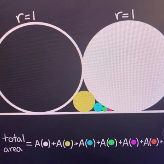
An infinite sequence of circles.
Suppose two circles with radius are just touching, and between them is a smaller (yellow) circle exactly fitting between them, an even smaller (blue) circle that touches the large circle on the right and the yellow circle, and so on. What is the total combined area of the circles?
The answer to this will take us to the zeta function, which connects geometry to prime numbers, quantum physics, and patterns in nature. It is the basis of the Riemann hypothesis about the distribution of prime numbers, appears in Planck’s blackbody radiation law and the Stefan-Boltzmann Law (see Economics and the Stefan Boltzmann Law and Stefan-Boltzmann Revisited), and provides a new perspective on the Cesàro sum we considered earlier in Extending Time where we saw a link to the physics of string theory.
Pell’s equation, introduced in Haven’s Haven, is a result in number theory that has connections to the zeta function, while Zipf’s Law, which governs word frequencies and city populations, can be viewed as a probability distribution when normalized by the zeta function. Seemingly unrelated problems across mathematics and physics often share deep underlying connections, with the zeta function serving as the thread that ties them together.
The geometry problem
Let’s start with the yellow circle with an unknown radius, .
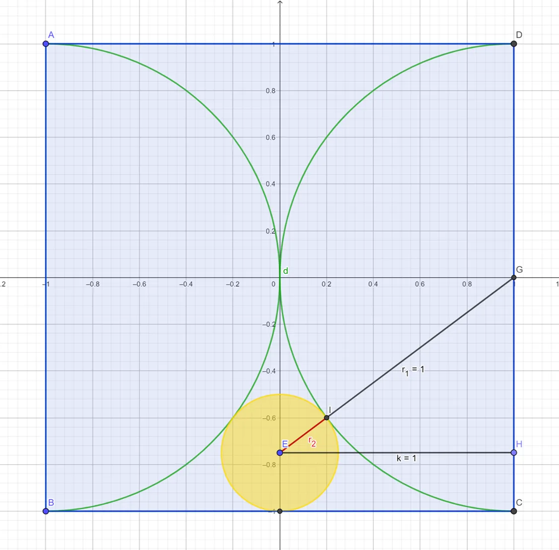
The yellow circle, .
If we construct a triangle with vertices such that is a right angle, then the length of the bottom side since it is the radius, of the large circle, the length of the side and the hypotenuse From the Pythagorean theorem,
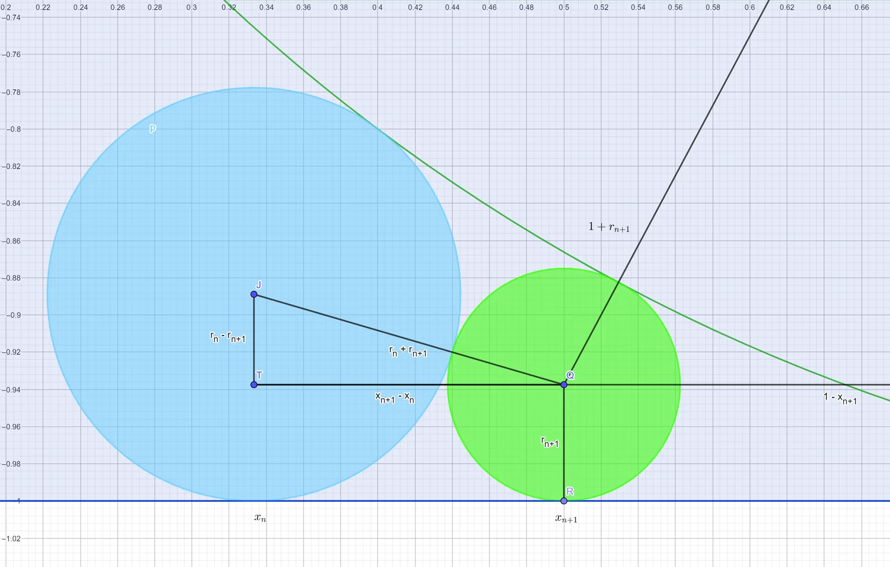
Now, let’s add the blue circle tucked in between the large circle and the yellow circle. The center of the blue circle is
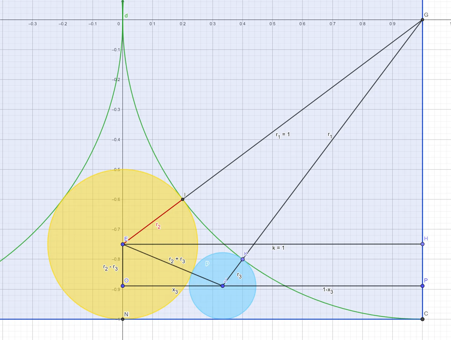
Locating the center of the blue circle.
We don’t know the coordinates of the blue circle yet, but we have two right-angle triangles. The first is and the second is From the first triangle,
Since we found that , then Using the Pythagorean theorem on and recalling that
For convenience, let be the distance along the axis from the center of the blue circle to the right edge of the square. Apply the substitution in the second-to-last step, and since represents a distance, we can discard the negative root, so
First Circles
The radius and position of the circle.
Suppose we know the position on the axis of the circle, and we know the radius . Using the method above, can we find the coordinates of the center of the next circle, We have two formulas using the Pythagorean theorem from the previous circle and from the first, large circle. The first,
The second uses the original large semicircle and the new circle,
Solving for , the discriminant is , so
Since and we can discard the negative root, so
From this, we can solve for the radius of the new circle,
Let’s check the formula using the yellow circle to find the blue circle. Since and we get
The next circle is the green one with center at , and from we get
The values for the axis positions () and radii () for each successive circle are determined by the formulas found in the last section, but simplifying the solutions can be tedious. Instead of calculating them by hand, let’s use Mathematica to find the answers. By putting the formulas in a loop, we can quickly generate a table of positions and radii for each circle.
Table: Circle positions and radii
Proof by Induction
The pattern for seems to be , and so we might hypothesize that and . To prove that this formula holds in general, we can use Proof by Induction. First, you show that the formula holds for an initial case, and then you show that if it holds for the case, then it also holds for the case.
To do this, we need to substitute the values for and into
and show that the formula is still valid. Let’s check this for the case where and The formula says
Next, we can check the formula for ,
The next step is to check the general case ,
and
And that’s it - proof by induction.
From circles to the zeta function
Interestingly, the sum of their areas leads directly to a famous mathematical object, the zeta function. The area of a circle with radius is so to find the areas of all of the small circles, we need to calculate
This is very nearly the zeta function,
The only difference is that starts at for the circle problem, while the definition of the zeta function sums over all of the natural numbers, so we need to subtract one from the zeta function or include the two semicircles with radii to make them the same.
The closed form of the zeta function was first solved by Leonhard Euler in 1734 for , and is called the Basel problem, after the city where Euler lived at the time. Euler found that . For the circles problem, , so the sum of the areas of all of the circles is
including the large semicircles with radius .
The Riemann Hypothesis
Bernhard Riemann was a German mathematician
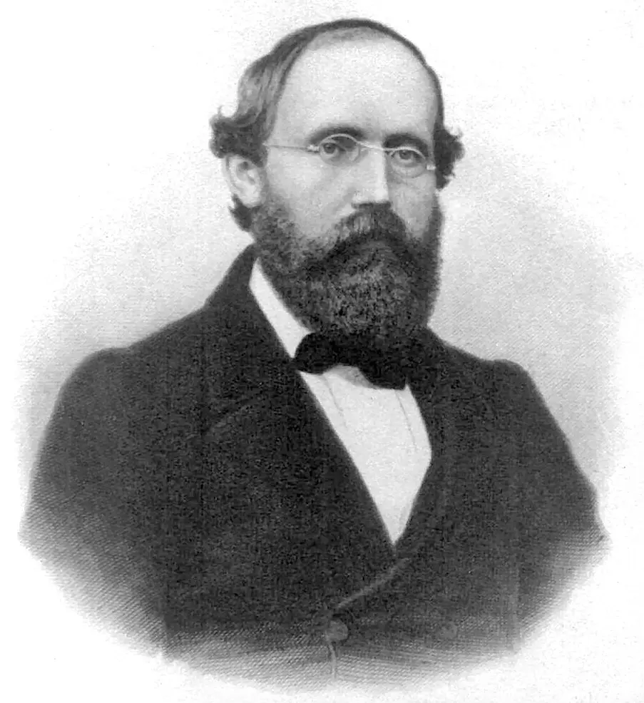
Georg Friedrich Bernhard Riemann.
who contributed significant new ideas to the areas of analysis, differential geometry, and number theory. He extended the zeta function through an analytic continuation A method for extending a function beyond its original domain while preserving its analytic properties. with the functional equation An equation that links a function’s values at different points (e.g., and ).,
The zeta function diverges when since it reduces to the harmonic series,
Riemann was interested in how the function behaved everywhere in the complex plane, that is, for all values of where For all values of , the zeta function diverges, so he extended it beyond the region where converges to other regions with a continuation. If two analytic functions agree on a connected region, their analytic continuation defines the same function everywhere that the function is valid.
Riemann began by expressing the series as an integral, using the Gamma function A continuation of factorials, is defined for all complex numbers except non-positive integers, and for positive integers.:
and substituted this into the zeta function to get
which converges everywhere except at He then derived the functional equation above that reflects the zeta function around the line so that the new function is defined everywhere in the complex plane except at But, while the functional equation relates to , it is not symmetric about the line in the complex plane. Riemann introduced the reflection formula for the Gamma function,
and substituted this into the functional equation to get the “completed” zeta function
which is symmetric since
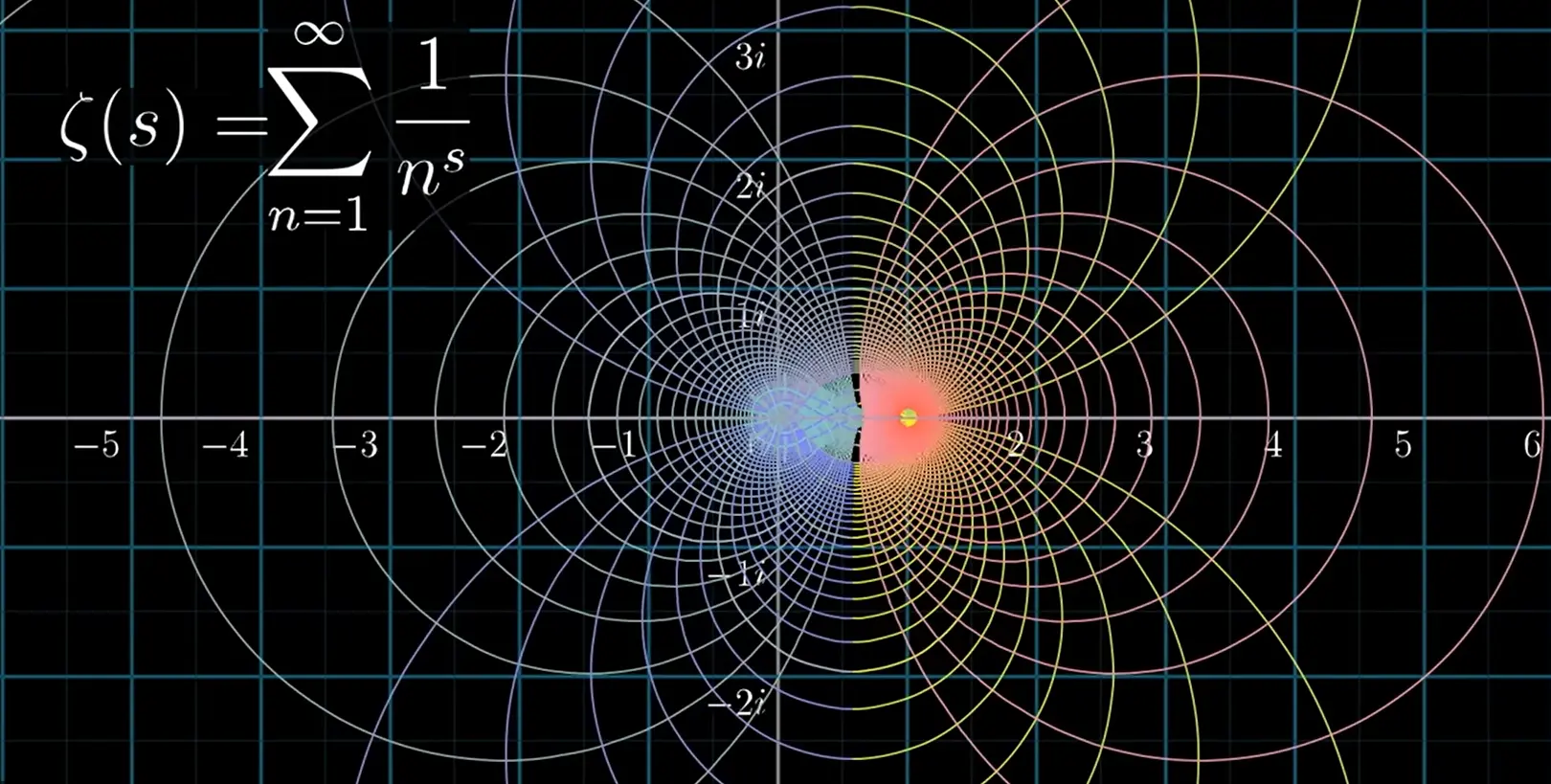
The analytic continuation of the function.
The line of symmetry where is very special because the analytic extension of has zeros along this line, that is, for some values of . In fact, three trillion zeros of the function have been found along this line, and none anywhere else except for the trivial cases of for where . What’s so important about this line? Well, the curious property of these zeros is that they can tell you where to find prime numbers.
A function called the prime pi function counts the number of primes less than some number. For example (using Pari/GP) primepi(10) = 4 because there are four primes less than , namely and The number of primes less than is primepi(1000) = 168. If you graph of this function you will see a step plot like this:

Prime counting function
Now, if you calculate the Riemann harmonic for any point in the complex plane,
and plot this for values of you get a curve like this:
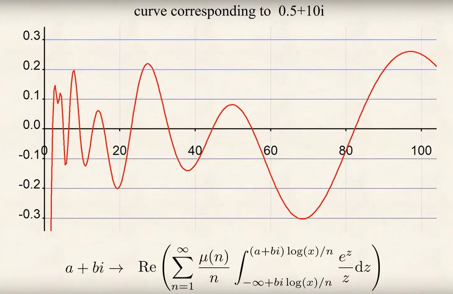
Riemann harmonic.
The function is the Möbius function, which is equal to if , if has squared prime factors, e.g., , and is equal to if is the product of distinct prime factors.
When you plot the Riemann harmonic (or Riemann Converter) at it generates a smooth curve:
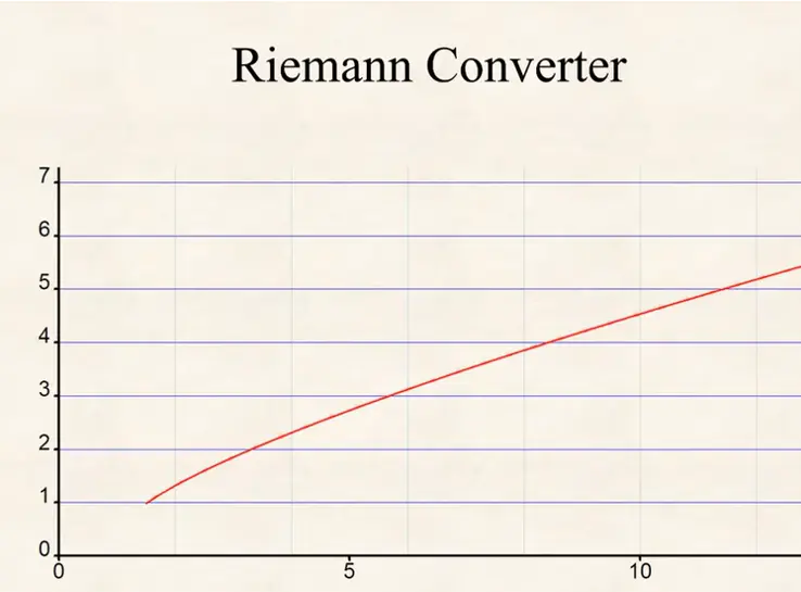
Riemann converter at .
Next, subtract the Riemann harmonic for each of the non-trivial zeros of from the curve at and we get this stair function:
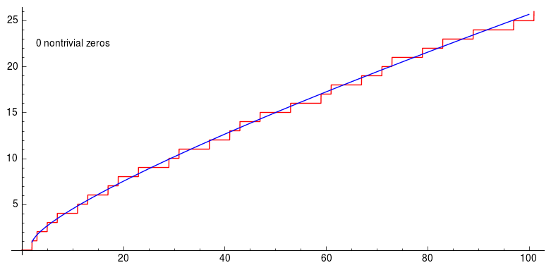
Riemann prime countinng formula.
which is exactly the prime counting formula! In other words, the Riemann zeta function tells us where to find primes even though they seem to be randomly distributed on the number line. Even though three trillion zeros of the zeta function have been found, nobody has a proof that they all lie on the line and nobody has found a counterexample. If you can do either, then the Clay Mathematics Institute would like to have a word with you and present you with a million dollars for solving one of the seven Millennium Prize Problems.
Planck, Stefan-Boltzmann, and Zeta
The solution to the circles problem required the particular value of , which coincidentally is also used in the derivation of Planck’s law of blackbody radiation. Blackbody radiation is the electromagnetic radiation emitted by an ideal, perfect absorber of all incident radiation, where the spectrum depends only on its temperature. This explains why objects glow at different colors as they heat up, like a heated piece of metal turning from red to white, and was central to the development of quantum theory because classical physics could not accurately describe it.
Before Planck, classical physics failed to explain the full black body spectrum, a problem known as the “ultraviolet catastrophe”. The classical Rayleigh-Jeans law correctly predicted the spectrum at long wavelengths but suggested that the radiation intensity would increase infinitely at higher frequencies, which did not match experimental observations.
The energy per unit volume per unit frequency of blackbody radiation at temperature is
where
- is the electromagnetic frequency of the radiation,
- is Planck’s constant, ,
- is the speed of light,
- is the Boltzmann constant, ,
- is the temperature in degrees Kelvin.
To find the total energy density , we need to integrate over all frequencies,
which may be simplified with a change of variables by letting
so that
and from the Riemann zeta function,
so, for the Planck equation, we need . Evaluating, and so
where and is the Stefan-Boltzmann constant,
The difference is in geometry - relates temperature to the radiation energy density while relates temperature to the radiative power per unit area giving the Stefan-Boltzmann law
that we used in Economics and the Stefan-Boltzmann Law and Stefan-Boltzmann Revisited.
Pell’s Equation
In Haven’s Haven, we introduced Pell’s equation
for a non-square positive integer , and developed an algorithm (The Chakravala) to find and satisfying the equation for a given . There are infinitely many solutions, and finding one solution reveals the others, but it can be difficult to find even the smallest. For example, when , the smallest values for and are and
By extending the number system to include a quadratic field A quadratic field extends rational numbers by adding , creating a new number system where expressions like become valid numbers with their own arithmetic rules., you get a modified version of the zeta function that’s specific to that extension. This modified zeta function gives how many numbers factor in the extended system and provides the fundamental unit, which is the smallest solution to the Pell equation.
The fundamental unit is the smallest unit greater than 1 in the ring of integers The ring of integers consists of all numbers in a field that satisfy polynomial equations with integer coefficients—think of it as the ‘whole numbers’ of an extended number system. of a real quadratic field. In real quadratic fields, units come from solutions to Pell’s equation since when , then is a unit or the multiplicative inverse of . That is,
Pell’s equation gives integer solutions, while the zeta function is a continuous, analytic function (except at ), but it provides discrete solutions just as it generates the prime counting function from the infinite sum of the continuous Riemann harmonics.
Zeta and Quantum Physics
In Extending Time, we showed how a consequence of Cesàro summation could lead to the result
or the sum of all natural numbers from 1 to is somehow Mathematica can calculate the values of for any using the built-in Zeta function, and Zeta[-1] returns which is equivalent to
so the sum works in the analytic continuation. Cesàro summation is used in string theory.
The command ComplexPlot3D[Zeta[z], {z, -2 - 2 I, 2 + 2 I}, PlotLegends -> Automatic] plots the zeta function over
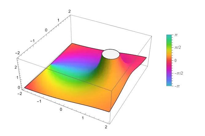
Plot of over .
See the JupyterLab Desktop for help setting up the Wolfram Language (Mathematica) in JupyterLab.
Zipf and Zeta
Zipf’s Law Zipf’s Law appears surprisingly often in nature and society, from word frequencies to city populations. It suggests an underlying simplicity in seemingly random distributions. (named for George Kingsley Zipf) says that frequency of occurrence is inversely proportional to rank. For example, the English word “the” occurs most often, appearing in about of written text, while the second most used word is “of”, which is found in of the text. This empirically derived law may be expressed as
Zipf’s Law applies to more than just word counts, as it has been found to describe the populations of cities, wealth inequality, and earthquakes.
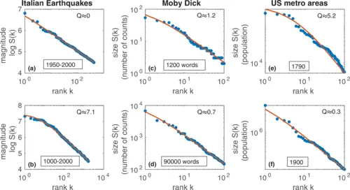
Zipf’s Law applied to earthquakes, word counts and city sizes.
Zipf’s Law says that the item on a list should have a frequency proportional to its rank raised to a power ,
and we can turn into a probability distribution by normalizing by the zeta function,
so that the sum over all probabilities is one, Even though Zipf’s Law is empirically derived, it is directly related to the zeta function and is found in a wide range of applications.
Summary
What began as a problem in geometry led to an exploration of prime numbers and the Riemann Hypothesis, connections to physics through Planck’s Law and the Stefan-Boltzmann Law of radiation, a look back at Cesàro sums and string theory, as well as an alternate perspective on Pell’s equation in number theory. Zipf’s Law, which finds wide application in linguistics, urban studies, and seismology, is directly related to the zeta function, which converts empirical observations into a probability distribution.
The zeta function appears in so many contexts because it captures something fundamental about how quantities scale and distribute—whether we’re counting primes, measuring radiation, or analyzing word frequencies. The mathematics of the zeta function weaves through number theory and physics, revealing deep connections between seemingly disparate phenomena.
Explore Further: Hands-On Experiments
The best way to develop intuition about the zeta function is to experiment with it yourself. Here are some concrete projects you can tackle with freely available tools:
- Explore Circle Packing in GeoGebra
- Download GeoGebra and recreate the nested circles problem.
- Use the formulas we derived to construct circles automatically.
- What happens if the two large circles have different radii? Can you derive a general formula?
- Try packing circles in other configurations—between three circles, or in a corner.
- Investigate the Zeta Function with PARI/GP
- Compute zeta values:
zeta(2),zeta(4),zeta(6)and verify they match the analytical formulas. - Create a special function
Z = lfuncreate(1)and then find the zeros less than 100,lfunzeros(Z,100). How would you verify that these are correct? - (Tricky) Experiment with Pell’s equation: Use
bnfinit(x^2-61)to explore the quadratic field and find the fundamental unit.
- Compute zeta values:
- Visualize with Mathematica/Wolfram Language
- Access through Wolfram Cloud (free tier available) or JupyterLab as described in our earlier article.
- Plot the zeta function:
Plot[Zeta[s], {s, -5, 5}]. - Verify the circle formula: Create a table comparing our analytical formula with numerical calculations.
- Test Zipf’s Law: Import a text file and count word frequencies, then plot log(rank) vs log(frequency) to see if it follows a power law.
- Prime Counting Experiments
- Use PARI/GP’s
primepi(x)function to count primes up to various limits. - Compare with the logarithmic integral approximation:
Li(x) = real(eint1(-log(x))). - For x = 100, 1000, 10000, compute the error:
primepi(x) - Li(x). Notice how the error oscillates—these oscillations are connected to the zeta zeros!
- Use PARI/GP’s
- Zipf’s Law Investigation
- Download any public domain text from Project Gutenberg.
- Write a simple word counter (or use existing tools) to get word frequencies.
- In Mathematica: Import the text, use
WordCounts[], then plot rank vs frequency on log-log axes. - Fit the data to a power law and extract the exponent .
- Try different types of texts (novels, technical works, poetry)—does the exponent change?
- Physics Connection
- Use the zeta function to verify the Stefan-Boltzmann constant.
- In Mathematica:
σ = (2 π^5 k^4)/(15 c^2 h^3)where k, c, h are the physical constants. - Compute the blackbody spectrum at different temperatures. How does Wien’s Law relate?
- Plot
u(ν,T)for T = 3000K, 5000K, 7000K to see why objects change color as they heat.
- Advanced Challenge: Riemann-Siegel Formula
- Implement a basic version of the Riemann-Siegel formula for computing ζ(1/2 + it).
- Use it to numerically search for zeros near the critical line
- Compare the results to the PARI/GP solution.
Code for this article
The Mathematica code Riemann_zeta.ipynb is contained in a JupyterLab Notebook, available on Github.
Software
- GeoGebra is dynamic mathematics software for all levels of education that brings together geometry, algebra, spreadsheets, graphing, statistics and calculus in one easy-to-use package.
- PARI/GP is a widely used computer algebra system designed for fast computations in number theory (factorizations, algebraic number theory, elliptic curves, modular forms, L functions…), but also contains a large number of other useful functions to compute with mathematical entities such as matrices, polynomials, power series, algebraic numbers etc., and a lot of transcendental functions.
- Wolfram Language is a symbolic language, deliberately designed with the breadth and unity needed to develop powerful programs quickly. By integrating high-level forms—like Image, GeoPolygon or Molecule—along with advanced superfunctions—such as ImageIdentify or ApplyReaction—Wolfram Language makes it possible to quickly express complex ideas in computational form.
References
[1] 3Blue1Brown - Visualizing the Riemann zeta function and analytic continuation. Accessed: Oct. 09, 2025.
[2] Michael Penn, A twist on a classic circle problem, (Nov. 24, 2024). Accessed: Oct. 08, 2025. [Online Video]. Available: https://www.youtube.com/watch?v=ZBTPG6dp_0U
[3] A. Bagdasaryan, An elementary and real approach to values of the Riemann zeta function, arXiv.org. Accessed: Oct. 12, 2025.
[4] G. H. Hardy, An Introduction To The Theory Of Numbers. Oxford New York Auckland: Oxford University Press, U.S.A., 2008.
[5] Basel problem, Wikipedia. Sept. 18, 2025. Accessed: Oct. 07, 2025.
[6] C. Shaw-Carmody, Computational Number Theory in Sage,
[7] J. M. Borwein, D. M. Bradley, and R. E. Crandall, Computational strategies for the Riemann zeta function, Journal of Computational and Applied Mathematics, vol. 121, no. 1, pp. 247–296, Sept. 2000, doi: 10.1016/S0377-0427(00)00336-8.
[8] Does the ‘Rich-Get-Richer’ Power-Law Truly Model Wealth Distribution? Accessed: Oct. 12, 2025.
[9] G. De Marzo, A. Gabrielli, A. Zaccaria, and L. Pietronero, Dynamical approach to Zipf’s law, Phys. Rev. Res., vol. 3, no. 1, p. 013084, Jan. 2021, doi: 10.1103/PhysRevResearch.3.013084.
[10] H. Montgomery, A. Nikeghbali, and M. T. Rassias, Eds., Exploring the Riemann Zeta Function: 190 years from Riemann’s Birth. Cham: Springer, 2017.
[11] L. Chiou, Fractal Chaos Discovered in Prime Numbers, Scientific American. Accessed: Oct. 07, 2025.
[12] J. Havil and F. Dyson, Gamma: Exploring Euler’s Constant. Princeton, N.J: Princeton University Press, 2009.
[13] A. Kontorovich, How I Learned to Love and Fear the Riemann Hypothesis, Quanta Magazine. Accessed: Oct. 08, 2025.
[14] D. J. Hutama, Implementation of Riemann’s Explicit Formula for Rational and Gaussian Primes in Sage.
[15] T. M. Apostol, Introduction to Analytic Number Theory. New York: Springer, 1976.
[16] Millennium Prize Problems, Wikipedia. Sept. 27, 2025. Accessed: Oct. 09, 2025.
[17] E. W. Weisstein, Möbius Function. Accessed: Oct. 10, 2025.
[18] Networks, Crowds, and Markets: A Book by David Easley and Jon Kleinberg. Accessed: Oct. 13, 2025.
[19] M. J. Mossinghoff and T. S. Trudgian, Nonnegative trigonometric polynomials and a zero-free region for the Riemann zeta-function, Journal of Number Theory, vol. 157, pp. 329–349, Dec. 2015, doi: 10.1016/j.jnt.2015.05.010.
[20] W. Dittrich, On Riemann’s Paper, ‘On the Number of Primes Less Than a Given Magnitude,’ Aug. 02, 2017, arXiv: arXiv:1609.02301. doi: 10.48550/arXiv.1609.02301.
[21] J. Derbyshire, Prime Obsession: Bernhard Riemann and the Greatest Unsolved Problem in Mathematics. New York: Plume, 2004.
[22] Prime-counting function, Wikipedia. Oct. 04, 2025. Accessed: Oct. 09, 2025.
[23] D. Hutama, Riemann explicit formula for primes. (July 04, 2025). Python. Accessed: Oct. 09, 2025.
[24] H. M. Edwards, Riemann’s Zeta Function. Mineola, NY: Dover Publications, 2001.
[25] D. N. Rockmore, Stalking the Riemann hypothesis: the quest to find the hidden law of prime numbers, 1. ed. New York, NY: Pantheon Books, 2005.
[26] A. E. Ingham, The Distribution of Prime Numbers. Cambridge ; New York: Cambridge University Press, 1990.
[27] The Euler-Maclaurin formula, Bernoulli numbers, the zeta function, and real-variable analytic continuation, What’s new. Accessed: Oct. 09, 2025.
[28] The Millennium Prize Problems, Clay Mathematics Institute. Accessed: Oct. 10, 2025.
[29] M. du Sautoy, The Music of the Primes: Searching to Solve the Greatest Mystery in Mathematics. New York: Harper Perennial, 2004.
[30] D. Platt and T. Trudgian, The Riemann hypothesis is true up to , Bulletin of London Math Soc, vol. 53, no. 3, pp. 792–797, June 2021, doi: 10.1112/blms.12460.
[31] J. Sondow, The Riemann Hypothesis, simple zeros and the asymptotic convergence degree of improper Riemann sums, Proc. Amer. Math. Soc., vol. 126, no. 5, pp. 1311–1314, 1998, doi: 10.1090/S0002-9939-98-04607-3.
[32] P. Borwein, S. Choi, B. Rooney, and A. Weirathmueller, Eds., The Riemann Hypothesis: A Resource for the Afficionado and Virtuoso Alike. New York ; London: Springer, 2008.
[33] The Riemann Zeros and Eigenvalue Asymptotics | SIAM Review. Accessed: Oct. 12, 2025.
[34] G. Lowther, The Riemann Zeta Function and the Functional Equation, Almost Sure. Accessed: Oct. 12, 2025.
[35] A. Ivic, The Riemann Zeta-Function: Theory and Applications. Mineola, N.Y: Dover Publications, 2003.
[36] A. R. Booker, Turing and the Riemann Hypothesis.
[37] T. Needham and R. Penrose, Visual Complex Analysis: 25th Anniversary Edition. Oxford, United Kingdom ; New York, NY: Oxford University Press, 2023.
[38] HexagonVideos, What is the Riemann Hypothesis REALLY about?, (Dec. 12, 2022). Accessed: Oct. 09, 2025. [Online Video]. Available: https://www.youtube.com/watch?v=e4kOh7qlsM4
[39] Zeta Functions: Dedekind Versus Hasse-Weil. Accessed: Oct. 12, 2025.
[40] Zipf’s law, Wikipedia. Oct. 06, 2025. Accessed: Oct. 12, 2025.
[41] Zipf’s Law for Cities – A Simple Explanation for Urban Populations : Networks Course blog for INFO 2040/CS 2850/Econ 2040/SOC 2090. Accessed: Oct. 12, 2025.
[42] S. T. Piantadosi, Zipf’s word frequency law in natural language: A critical review and future directions, Psychon Bull Rev, vol. 21, no. 5, pp. 1112–1130, Oct. 2014, doi: 10.3758/s13423-014-0585-6.
Image credits
- Hero image: Turtles All The Way Down, Polymathic Being
- An infinite sequence of circles: Classical Mathematics Group, David Rattner, December 2, 2024.
- Geometric graphs: Geogebra.
- Georg Friedrich Bernhard Riemann photo: By http://www.sil.si.edu/digitalcollections/hst/scientific-identity/explore.htm according to the German Wikipedia., Public Domain, https://commons.wikimedia.org/w/index.php?curid=27383
- The analytic continuation of the function - But what is the Riemann zeta function? Visualizing analytic continuation. Grant Sanderson, 3Blue1Brown.
- Prime counting function, Riemann Converter - What is the Riemann Hypothesis REALLY about?. HexagonVideos.
- Pi 100 - Prime Pages.
- Riemann’s explicit formula using the first 200 non-trivial zeros of the zeta function - By Daniel Hutama.
- Zeta surface plot: Mathematica.
- Zipf’s Law - Dynamical approach to Zipf’s law.